1.easygui

easygui是Python的一个图形化界面的库。
下载模块
```
pip install easygui
```

常用功能

消息弹窗

msgbox()   #消息弹窗
msgbox(msg=' ', title=' ', ok_button=' ', image=None, root=None)
msg：#需要显示的内容
title：#窗口的标题
ok_button：#按钮上显示的信息
image：#显示图片（需要路径）
#返回值：
 #按钮信息
 #右上角×号返回None
#########################
import easygui as t
t.msgbox('Hello','easy','Yes','wjx.png')

双项选择

ccbox()     #双项选择
ccbox(msg=' ', title=' ', choices=('  ', '  '), image=None)
msg：#需要显示的内容
title：#窗口的标题
choices：#元组形式，两个选项显示的内容
image：#显示图片（需要路径）

#返回值：
 #第一个按钮返回True
 #第二个按钮返回False
 #右上角×号返回None

import easygui as t
t.ccbox('下面水果，你喜欢哪一个？','选择',('苹果','橘子'))

多项选择

buttonbox()   #多项选择
buttonbox(msg=' ', title=' ', choices=('Button1', 'Button2', 'Button3'), image=None, root=None)

msg：#需要显示的内容
title：#窗口的标题
choices：#元组形式或列表的形式，多个选项显示的内容
image：#显示图片（需要路径）

#返回值：
 #点击按钮返回按钮的信息
 #右上角×号返回None

import easygui as t
tuple = ('石头','剪刀','布')
t.buttonbox('选择石头剪刀布','game',tuple)

可选的下拉列表

choicebox()与multchoicebox()——#可选的下拉列表
choicebox(msg=' ', title=' ', choices=())
msg：#需要显示的内容
title：#窗口的标题
choices：#元组形式或列表的形式，多个选项显示的内容

#返回值：
 #点击显示的选项，返回选项的信息
# 点击Cancel按钮返回None
# 右上角×号返回None

import easygui as t
list = ['石头','剪刀','布']
t.choicebox('选择石头剪刀布','game',list)

multchoicebox()#功能同样，只是他可以提供多选，拥有全选与全清按钮。

#返回值：
# 多选的返回值是多选的文本列表
# 点击Cancel按钮返回None
# 右上角×号返回None

文本输入框

enterbox()    #文本输入框
enterbox(msg='  ', title=' ', default=' ', strip=True, image=None, root=None)
msg：#需要显示的内容
title：#窗口的标题
default：#关键字定义的是文本框默认值
strip：#的值为True时会自动忽略输入的首尾空格，False则相反
image：#显示图片（需要路径）

#返回值：
## 输入内容后返回值为输入的字符串
#点击Cancel按钮返回None
 #右上角×号返回None
   
import easygui as t
s = t.enterbox('What do you want to say ?','想说什么','Who are you ?')
print(s)

数字输入

integerbox() #  数字输入
integerbox(msg='', title=' ', default='', lowerbound=0, upperbound=99, image=None, root=None,)
msg：#需要显示的内容
title：#窗口的标题
default：#关键字定义的是文本框默认值
lowerbound：#输入的最小值
upperbound：#输入的最大值
image：#显示图片（需要路径）

#返回值：
# 输入内容后返回值为输入的数字
# 点击Cancel按钮返回None
# 右上角×号返回None
#输入数值超出范围时会给出提示后从新输入。

import easygui as t
s = t.integerbox('你多大了','年龄','18',0,120)
print(s)

多选项输入

mulenterbox()  #多选项输入
multenterbox(msg=' ', title=' ', fields=(), values=())
msg：#需要显示的内容
title：#窗口的标题
fields：#填写条目名称
values：#默认内容

#返回值：
### 输入内容后返回值为输入的内容，以列表的形式
# 点击Cancel按钮返回None
## 右上角×号返回None

import easygui as t
message = ['学号', '姓名','性别','年龄','院系','入学时间']
s = student = t.multenterbox('输入学生的信息：', '信息录入', message)
print(s)

密码输入框

passwordbox()#密码输入框（不显示）
passwordbox(msg=' ', title=' ', default=' ', image=None, root=None)
msg：#需要显示的内容
title：#窗口的标题
default：#关键字定义的是文本框默认值
image：#显示图片（需要路径）

#返回值：
# 输入内容后返回值为输入的字符串
## 点击Cancel按钮返回None
# 右上角×号返回None

import easygui as t
s = t.passwordbox('输入密码', '密码')
print(s)

多项显示

multpasswordbox() #多项显示
multpasswordbok(msg=' ', title=' ',fields=(),values=())
msg：#需要显示的内容
title：#窗口的标题
fields：#填写条目名称，最后一栏显示为*号
values：#默认内容

#返回值：
# 输入内容后返回值为输入的内容，以列表的形式
# 点击Cancel按钮返回None
# 右上角×号返回None

import easygui as t
s = t.multpasswordbox('请输入账号密码', '登录',['用户名','账号','密码'],['123','123','123'])
print(s)

2.openpyxl

安装模块
```
pip install openpyxl
```

常用功能

1.sheet

from openpyxl import load_workbook

#打开excel文件
workbook = load_workbook("文件名")

#1.获取所有的sheet名称
name_list = workbook.sheetnames
print(name_list)

#2.根据名称获取sheet
sheet_object = workbook["sheetname"]
print(sheet_object)

#3.根据索引获取sheet
sheet = worksheets[0]

#4.循环获取所有的sheet
for sheet_object in wcrkbook:
    print(sheet_object)
#不加.sheetnames内部也是自动获取sheetnames的

2.sheet中单元格的数据

from openpyxl import load_workbook

workbook = load_workbook("文件路径")
sheet = workbook.worksheets[1]

#1.获取 第n行 &第n列 的单元格(起始位置是1)
cell = sheet.cell(1,1)
print(cell)
print("内容",cell.value)
print("样式",cell.style)
print("字体",cell.font)
print("排序",cell.alignment)

#2.根据Excel的位置获取数据
cell_al = sheet["A1"]
print(cell_al.value)

#3.获取第n行的单元格
cell_list = sheet[1]

for cell in sheet[1]:
    print(cell.value)
    
#4.循环获取所有行数据
for row in sheet.rows:
    print(row[0].value)
    
#5.循环获取所有列
for col in sheet.columns:
    print(col[0].value)

3.合并的单元格

from openpyxl import load_workbook

workbook = load_workbook("文件路径")
sheet = workbooks[2]

#1.获取单元格
c1 = sheet.cell(1,1)
print(c1) #<cell "Sheet1".A1>
print(c1.value) #用户信息
#第一个和第二个合并单元格，第一个显示值，第二个显示null
c1 = sheet.cell(1,2)
print(c1) #<MergedCell "Sheet1".B1>
print(c1.value) #None

4.Excel

4.1原Excel文件基础上写内容

from openpyxl import load_workbook

workbook = load_workbook("文件路径")
sheet = worksheets[0]

#1.找到单元格，并修改单元格的内容
cell = sheet.cell(1,1)
cell.value = "值"

#将excel文件保存到p2.xlsx文件中
workbook.save("文件路径")

4.2新创建Excel文件写内容

from openpyxl import workbook

#创建excel且默认会创建一个sheet（名称为sheet）
workbook = workbook.Workbook()

sheet = worksheets[0]

#找到单元格，并修改单元格的内容
cell = sheet.cell(1,1)
cell.value = "值"

#将excel文件保存到p2.xlsx文件中
workbook.save("文件路径")

4.3删除和修改

from openpyxl import workbook

workbook = workbook.workbook()

#1.修改sheet名称
sheet = worksheets[0]
sheet.title = "值"
workbook.save("p2.xlsx")

#2.创建sheet并设置sheet颜色
sheet = workbook.create_sheet("工作计划",0)#零代表位置
sheet.sheet_properties.tabColor = "1072BA"
workbook.save("P2.xlsx")

#3.默认打开的sheet
workbook.active = 0
workbook.save("p2.xlsx")

#4.拷贝sheet
sheet = workbook.create_sheet("工作计划")
sheet.sheet_properties.tabColor = "1072BA"

new_sheet = workbook.copy_worksheet(workbook["Sheet"])
new_sheet.title = "新的计划"
workbook.save("p2.xlsx")

#5.删除sheet
del workbook["用户列表"]
workbook.save("files/p2.xlsx")

5.操作单元格

from openpyxl import load_workbook
from openpyxl.styles import Alignment,Border,Side,Font,PatternFill,GradientFill

workbook = load_workbook("文件")
sheet = workbook.worksheet[1]
#1.获取某个单元格，修改值
cell = sheet.cell(1,1)
cell.value = "开始"

#2.获取某个单元格，修改值
sheet["V3"] = "Alex"
vb.save("p2.xlsx")

#3.获取某些单元格，修改值
cell_list = sheet[B2:C3]
#b2到c3拿到的值是(b2,b3,c2,c3)
for row in cell_list:
    for cell in row :
        cell.value = "新的值"
vb.save("p2.xlsx")

#4.对齐方式
cell = sheet.cell(1,1)
#herizontal,水平方向对齐方式：“general”,"left","center"句中,"right","fill","justify","centercontinuous","distributed"
#vertieal,垂直方向对齐方式："top","center","bottom","justify","distributed"
#text_rotation,旋转角度
#wrap_text,是否自动换行
cell.alignment = Alignment(horizontal="center",vertical="distributed",text_rotation=45,wrap_text=True)
wb.save("p2.xlsx")

#5.边框
#side的style有如下：dashDot,dashDotDot,dashed,dotted,double,hair,mediun,mediumDashDot,mediumDashDotdot,mediumDashed,slantDashDot,thick,thin.
sell = sheet.cell(9.2)
cell.border = Border(
	top = Side(style="thin",color="FFB6C1"),   
    bottom=Side(style="dashed",color="9932cc"),
    left=Side(style="dashed",color="9932cc"),
    right=Side(style="dashed",color="9932cc"),
    diagonal=Side(style="thin",color="483D8B"),#对角线
    diagonalUp=True,#左下-右上
    #diagonalDown=True #左上-右下
)
wb.save("p2.xlsx")

#6.字体
cell = sheet.cell(5,1)
cell.font = Font(name="微软雅黑",size=45，color="ff0000",underline="single") #underline下划线
wb.save("p2.xlsx")

#7.背景色
cell = sheet.cell(5,3)
cell.fill = PatternFill("solid",fgColor="99ccff")
wb.save("p2.xlsx")

#8.渐变背景色
cell = sheet.cell(5,5)
cell.fill = GradientFill("linear",stop=("FFFFFF","99ccff","000000"))#从左到右的三个颜色
wb.save("p2.xlsx")

#9.宽高（索引从1开始）
sheet.row_idmensions[1].height = 50
sheet.column_dimensions["E"].width = 100
wb.save("p2.xlsx")

#10.合并单元格
sheet.merge_cells("B2:D8")
#这是两种
sheet.merge_cells(start_row=15,start_column=3,end_row=18,end_column=8)
wb.save("p2.xlsx")
#这是解除合并单元格的
sheet.unmerge_cells("B2:D8")
wb.save("p2.xlsx")

#11.写入公式
sheet = wb.worksheets[3]
sheet["D1"] = "合计"
sheet["D2"] = "=B2*C2"
wb.save("p2.xlsx")

sheet = wb.worksheets[3]
sheet["D3"] = "=sum(B3,C3)"
wb.save("p2.xlsx")

#12.删除
#idx,要删除的索引位置
#anount,从索引位置开始要删除的个数(默认为1)
sheet.delete_rows(idx=1,anount=2)
sheet.delete_cols(idx=1,anount=3)
wb.save("p2.xlsx")

#13.插入
sheet.insert_rows(idx=5,anount=10)
sheet.insert_cols(idx=3,anount=2)
wb.save("p2.xlsx")

#14.循环写内容

sheet = wb["Sheet"]
cell_range = sheet["A1:C2"]
for row in cell_range:
    for cell in row:
        cell.value = "xx"
#第5行第1列到第7行第10列
for row in sheet.iter_rows(min_row=5,min_col=1,max_col=7,max_row=10):
    for cell in row:
        cell.value = "oo"
wb.save("p2.xlsx")

#15.移动
#将H2:J10范围的数据，向右移动15个位置、向上移动1个位置
sheet.nove_range("H2:J10",rows=-1,cols=15)
wb.save("p2.xlsx")

#16.打印区域
sheet.print_area = "A1:D200"
wb.save("p2.xlsx")

#17.打印时，每个页面的固定表头
sheet.print_title_cols = "A:D"
sheet.print_title_rows = "1:3"
wb.save("p2.xlsx")

6.作业

补充代码：实现去网上获取指定地区的天气信息，并写入excel中。

import requests

while True:
    city = input("请输入城市（Q/q退出）：")
    if city.upper()=="Q":
        break
    url = "http://ws.webxml.com.cn//webServices/WeatherWebService.asmx/getWeatherbyCityName?theCityName={}".format(city)
    res = requests.get(url=url)
    print(res.text)
    
    #1.提取xml格式中的数据
    #2.为每个城市创建一个sheet，并将获取的xml格式中的数据写入到excel中。
    from openpyxl import load_workbook

        workbook = load_workbook("a1.xlsx")
        sheet = workbook.create_sheet("工作计划")
        sheet.title = city
        sheet = workbook[city]
        cell=sheet["A1:AH1"]
        text=str(res.text)[:-16].split("<string>")[1:]
        for i in range(len(text)):
            cell[0][i].value = text[i][:-13]
            print(text[i][:-13])
        workbook.save("a1.xlsx")

读取ini文件内容,按照规则写入到Excel中

[mysqld]
datadir=/var/lib/mysql
socket=py-mysql-bin
log-bin=py-mysql-bin
character-set-server=utf8
collation-server=utf8_general-ci
log-error=/var/log/mysqld.log
symbolic-links=0

[mysqld_safe]
log-error=/var/log/mariadb/mariadb/mariadb.log
pid-file=/var/run/mariadb/mariadb.pid

[client]
default-character-set=utf8
#1.读取ini格式的文件，并创建一个excel文件，并且每个节点创建一个sheet，然后将节点下的键值写入到excel中。
#2.首行，字体白色&单元格背景色蓝色
#3.内容均句中
#4.边框

3.Matplotlib and Plotly

安装 Matplotlib and Plotly

pip install matplotlib
pip install Plotly

1.Matplotlib

基本使用

import matplotlib.pyplot as plt
from matplotlib.font_manager import FontProperties

x_values = range(1, 1001, 19)
y_values = [x**2 for x in x_values]						# 自动计算数据

# 写上这两行后可以解决，字体无法显示的问题。
plt.rcParams['font.sans-serif']=['SimHei']
plt.rcParams['axes.unicode_minus'] = False

# print(plt.style.available) 								# 查看样式
plt.style.use("Solarize_Light2") 						# 网格样式
fig, ax = plt.subplots()

# 隐藏xy轴，写这个可以隐藏坐标轴
# ax.get_xaxis().set_visible(False)
# ax.get_yaxis().set_visible(False)

ax.scatter(x_values, y_values, c="red", s=1)			# 调用scatter()并使用参数s设置绘制图形时使用的点的尺寸,c是颜色。
# ax.scatter(x_values, y_values, c=y_values, cmap=plt.cm.Blues, s=100)
# c是颜色,写数据是透明色的透明度，cmap=plt.cm.Blues是告诉pyplot使用什么渐变颜色

ax.set_title("平方数", fontsize=24)                      # 表标题，字号24
ax.set_xlabel("值", fontsize=14)						# x轴标题，字号14
ax.set_ylabel("值的平方", fontsize=14)					# y轴标题，字号14

ax.tick_params(axis="both", which="major", labelsize=14)  # 设置刻度标记的大小。
ax.axis([0, 1100, 0, 1100000])								# 设置每个坐标轴的取值范围

# plt.savefig("squares_plot.png", bbox_inches="tight")  # 这个方法是用来保存图片的，第一个参数是图片的名称，第二个是去掉多余的白边，
plt.show()

将数据以逗号翻个的称为CSV文件，对人阅读比较麻烦，但是程序可以轻松提取并处理。

import csv
from datetime import datetime
import matplotlib.pyplot as plt

with open("aa.csv") as f:
    reader = csv.reader(f)				#将存储的对象最为实参
    header_row = next(reader)			#传入阅读器对象时，它将返回文件中的下一行
   	# for index,column_header in enumerate(header_row):	# enumerate用于获取索引及其值
    #     print(index,column_header)
    dates, highs, lows = [], [], []
    for row in reader:			#循环获取
        current_date = datetime.strptime(row[2], "%Y-%m-%d")		#索引获取时间并转为时间类型
        # 时间参数还有很多
        # %A    星期几，%B    英文月份名，%m    数字月份名，%d    数字天数，
        # %Y    四位年份，%y    两位年份，%H    24小时制小时数，%I    12小时制小时数，
        # %p    am或pm，%M    分钟数，%S    秒数
        try:
            high = int(row[5])		#获取索引5处的数据
            low = int(row[6])
        except ValueError:			#在天气的之中会出现没有值的情况，刚好ValueError可以检测到这个错误。
        	print(f"Missing data for {current_date}")
        else:
            dates.append(current_date)
            highs.append(high)
            lows.append(low)

plt.rcParams['font.sans-serif']=['SimHei']
plt.rcParams['axes.unicode_minus'] = False

plt.style.use("seaborn")
fig,ax = plt.subplots()
ax.plot(dates, highs, C="red", alpha=0.5)		# alpha透明度，0透明，1不透明。
ax.plot(dates, lows, C="blue", alpha=0.5)
ax.fill_between(dates,highs,lows,facecolor="blue",alpha=0.1) #x,y,y,facecolo颜色， alpha透明度，0透明，1不透明。

ax.set_title("2018年7月每日最高气温", fontsize=24)
ax.set_xlabel("", fontsize=14)
fig.autofmt_xdate()						# 绘制倾斜的标签
ax.set_ylabel("温度", fontsize=14)

plt.show()

2.Plotly

基本使用

from random import randint

class Die:
    def __init__(self, num_sides=6):
        self.num_sides = num_sides
    def roll(self):
        return randint(1, self.num_sides)		# randiint用于生成随机数
        
die1 = Die()
die2 = Die()

results = [die1.roll()+die2.roll() for roll_num in range(100)]
frequencies = [results.count(value) for value in range(1, (die1.num_sides+die2.num_sides)+1)]
print(results)
print(frequencies)
# 绘制直方图
from plotly.graph_objs import Bar,Layout
from plotly import offline

x_values = list(range(2, (die1.num_sides+die2.num_sides)+1))
data = [Bar(x=x_values, y=frequencies)]				# 收集数据

x_axis_config = {"title":"结果","dtick":1}		   # x标题及属性设置,dtick是刻度间距
y_axis_config = {"title":"结果的频率"}				 # y标题及属性设置
my_layout = Layout(title="2骰子1000次的结果", xaxis=x_axis_config, yaxis=y_axis_config)	# 标题整理
offline.plot({"data":data,"layout":my_layout}, filename="d6.html")		# 渲染并保存

json是使用非常广泛的数据格式。

import json
import plotly.express as px

"""
print(px.colors.named_colorscales())		#这个方法可以查看，可以使用的渐变。
"""

with open("bbb.json") as f:
    all_eq_data = json.load(f)			# load用于将json转为可以处理的格式
""" 
with open("ccc.json","w") as f:
    json.dump(all_eq_data,f,indent=4)	# dump接收一个json数据和一个文件数据，indent用于结构匹配的缩进。
"""   
all_eq_dicts = all_eq_data["features"]
mags, titles, lons, lats = list(), list(), list(), list()
for eq_dict in all_eq_dicts:
    mag = eq_dict["properties"]["mag"]
    title = eq_dict["properties"]["title"]
    lon = eq_dict["geometry"]["coordinates"][0]
    lat = eq_dict["geometry"]["coordinates"][1]
    mags.append(mag)
    titles.append(title)
    lons.append(lon)
    lats.append(lat)
    
fig = px.scatter(
	x=lons,
    y=lats,
    labels={"x":"经度","y":"纬度"},
   	range_x=[-200,200]		#范围
   	range_y=[-90,90]
    width=800,		#宽高800像素
    height=800,
    title="全球地震散点图",
    size = mags,	#默认点尺寸为20像素
    size_max=10,	#最大显示尺寸缩放到10
  	color = mags,	#设置渐变
    hover_name = titles	#震级大致位置
)	
fig.write_html("global_earthquakes.html")		# 保存
fig.show()	#查看

4.sys

sys模块提供了一系列有关Python运行环境的变量和函数。

sys.argv，可以获取当前正在执行的命令行参数的参数列表(list)。变量解释

sys.argv[0]当前程序名

sys.argv[1]第一个参数

sys.argv[2]第二个参数

len(sys.argv)-1 参数个数(减去文件名)

import sys
print(sys.argv)
print(sys.argv[0])
print(sys.argv[1])
print("第二个参数:%s"%sys.argv[2])
print("参数个数：%s"%(len(sys.argv)-1))
-------------------结果：
#python /root/mcw.py arg1 arg2
['/root/mcw.py', 'arg1', 'arg2']
/root/mcw.py    #当前程序名
arg1
第二个参数:arg2
参数个数：2
2）　如果执行用的相对路径，返回的是相对路径
print(sys.argv[0])
----------------结果：
[root@xiaoma /root] test!
#python ./mcw.py 
./mcw.py#sys.argv =['/root/mcw.py', 'arg1', 'arg2'] ，列表第一个元素为程序执行相对路径，第二个元素开始为程序传参

sys.path

返回模块的搜索路径，初始化时使用PYTHONPATH环境变量的值

import sys
print(sys.path)
---------------------结果：
['D:\\aPython_full目录\\小马过河的代码练习', 'C:\\mcw', 'C:\\mcw\\venv\\Scripts\\python36.zip', 'C:\\python3\\DLLs', 'C:\\python3\\lib', 'C:\\python3', 'C:\\mcw\\venv', 'C:\\mcw\\venv\\lib\\site-packages', 'C:\\mcw\\venv\\lib\\site-packages\\setuptools-39.1.0-py3.6.egg', 'C:\\mcw\\venv\\lib\\site-packages\\pip-10.0.1-py3.6.egg', 'C:\\软件安装\\PyCharm 2018.3.5\\helpers\\pycharm_matplotlib_backend']

添加系统环境变量：
import sys,os

BASE_DIR = os.path.dirname(os.path.dirname(os.path.abspath(__file__)))
print(BASE_DIR)
#添加系统环境变量
sys.path.append(BASE_DIR)
print(sys.path)

import sys
sys.path.append("C:\python3\Scripts")
print(sys.path)
------------------结果：
['D:\\.........., 'C:\\python3\\Scripts']

sys.platform

获取当前执行环境的平台，如win32表示是Windows系统，linux2表示是linux平台

print(sys.platform)
-------------结果：
win32  

-------------结果：
[root@xiaoma /root] test!
#python mcw.py 
linux2

sys.exit(n)

调用sys.exit(n)可以中途退出程序，当参数非0时，会引发一个SystemExit异常，从而可以在主程序中捕获该异常。
```
#vim mcw.py 
import sys
sys.exit(3)
----------结果：
[root@xiaoma /root] test!
#python mcw.py 
[root@xiaoma /root] test!
#echo $?
3
```

sys.version

获取Python解释程序的版本信息

import sys
print(sys.version)
--------------结果：
3.6.8 (tags/v3.6.8:3c6b436a57, Dec 23 2018, 23:31:17) [MSC v.1916 32 bit (Intel)]

import sys
print(sys.version)
--------------结果：
[root@xiaoma /root] test!
#python mcw.py 
2.7.5 (default, Nov  6 2016, 00:28:07) 
[GCC 4.8.5 20150623 (Red Hat 4.8.5-11)]

sys.getrefcount

获取一个值的应用计数

a = [11,22,33]
b = a
print(sys.getrefcount(a))
--------------结果：
3 #a,b，还有gerefcount方法三个都在使用这个列表

sys.getrecursionlimit python默认支持的递归数量
sys.stdout.write　　　　　可以做输出重定向
```
for i in range(3):
    print("魔降风云变")
import sys
for i in range(3):
    sys.stdout.write('小马过河')
-----------------结果：
魔降风云变
魔降风云变
魔降风云变
小马过河小马过河小马过河

import sys
for i in range(3):
    sys.stderr.write('小马过河')
------------------结果：
小马过河小马过河小马过河
```
stdout 是一个类文件对象；调用它的 write 函数可以打印出你给定的任何字符串。实际上，这就是 print 函数真正做的事情；它在你打印的字符串后面加上一个硬回车，然后调用 sys.stdout.write 函数。在最简单的例子中，stdout 和 stderr 把它们的输出发送到相同的地方和 stdout 一样，stderr 并不为你添加硬回车；如果需要，要自己加上。 stdout 和 stderr 都是类文件对象，但是它们都是只写的。它们都没有 read 方法，只有 write 方法。然而，它们仍然是类文件对象，因此你可以将其它任何 (类) 文件对象赋值给它们来重定向其输出。

sys.modules

import sys,os
print(sys.modules.keys())
-----------------------结果；
dict_keys(['builtins', 'sys', '_frozen_importlib', '_imp', '_warnings', '_thread', '_weakref', '_frozen_importlib_external', '_io', 'marshal', 'nt', 'winreg', 'zipimport', 'encodings', 'codecs', '_codecs', 'encodings.aliases', 'encodings.utf_8', '_signal', '__main__', 'encodings.latin_1', 'io', 'abc', '_weakrefset', 'site', 'os', 'errno', 'stat', '_stat', 'ntpath', 'genericpath', 'os.path', '_collections_abc', '_sitebuiltins', '_bootlocale', '_locale', 'encodings.gbk', '_codecs_cn', '_multibytecodec', 'sysconfig', 'encodings.cp437', 'sitecustomize'])

5.xlrd

1.背景

安装模板：

#到python官网下载http://pypi.python.org/pypi/xlrd模块安装，前提是已经安装了python 环境。
#在cmd命令行输入:pip install xlrd

xlrd介绍：xlrd是python环境下对excel中的数据进行读取的一个模板，可以进行的操作有：读取有效单元格的行数、列数

读取指定行（列）的所有单元格的值

读取指定单元格的值

读取指定单元格的数据类型

2.常用函数

打开文件（获取一个工作表）：

import xlrd
data = xlrd.open_workbook("01.xls")					# 打开当前目录下名为01.xls的文档
													#此时data相当于指向该文件的指针
table = data.sheet_by_index(0)						# 通过索引获取，例如打开第一个sheet表格
table = data.sheet_by_name("sheet1")				# 通过名称获取，如读取sheet1表单
table = data.sheets()[0]							# 通过索引顺序获取
													# 以上三个函数都会返回一个xlrd.sheet.Sheet()对象
names = data.sheet_names()    						# 返回book中所有工作表的名字
data.sheet_loaded(sheet_name or indx)   			# 检查某个sheet是否导入完毕

对行进行操作：

nrows = table.nrows  								# 获取该sheet中的有效行数
table.row(rowx)  									# 返回由该行中所有的单元格对象组成的列表
table.row_slice(rowx)  								# 返回由该列中所有的单元格对象组成的列表
table.row_types(rowx, start_colx=0, end_colx=None)  # 返回由该行中所有单元格的数据类型组成的列表
table.row_values(rowx, start_colx=0, end_colx=None) # 返回由该行中所有单元格的数据组成的列表
table.row_len(rowx) 								# 返回该列的有效单元格长度

对列进行操作：

ncols = table.ncols									# 获取列表的有效列数
table.col(colx, start_rowx=0, end_rowx=None)		# 返回由该列中所有的单元格对象组成的列表
table.col_slice(colx, start_rowx=0, end_rowx=None)	# 返回由该列中所有的单元格对象组成的列表
table.col_types(colx, start_rowx=0, end_rowx=None)	# 返回由该列中所有单元格的数据类型组成的列表
table.col_values(colx, start_rowx=0, end_rowx=None)	# 返回由该列中所有单元格的数据组成的列表

对单元格进行操作：

table.cell(rowx, colx)  							# 返回单元格对象
table.cell_type(rowx, colx)  						# 返回单元格中的数据类型
table.cell_value(rowx,colx)  						# 返回单元格中的数据

6.pygame

安装Pygame
```
pip install pygame
```

Pygame常用模块

模块名	功能
pygame.cdrom	访问光驱
pygame.cursors	加载光标
pygame.display	访问显示设备
pygame.draw	绘制形状、线和点
pygame.event	管理事件
pygame.font	使用字体
pygame.image	加载和存储图片
pygame.joystick	使用游戏手柄或者类似的东西
pygame.key	读取键盘按键
pygame.mixer	声音
pygame.mouse	鼠标
pygame.movie	播放视频
pygame.music	播放音频
pygame.overlay	访问高级视频叠加
pygame.rect	管理矩形区域
pygame.scrap	本地剪贴板访问
pygame.sndarray	操作声音数据
pygame.sprite	操作移动图像
pygame.surface	管理图像和屏幕
pygame.surfarray	管理点阵图像数据
pygame.time	管理时间和帧信息
pygame.transform	缩放和移动图像

简单示例：

import pygame
import sys

pygame.init()  # 初始化pygame
size = width, height = 320, 240  # 设置窗口大小
screen = pygame.display.set_mode(size)  # 显示窗口

while True:  # 死循环确保窗口一直显示
    for event in pygame.event.get():  # 遍历所有事件
        if event.type == pygame.QUIT:  # 如果单击关闭窗口，则退出
            sys.exit()
pygame.quit()  # 退出pygame

制作一个跳跃的小球游戏
- 创建一个游戏窗口，然后在窗口内创建一个小球。以一定的速度移动小球，当小球碰到游戏窗口的边缘时，小球弹回，继续运动按照如下步骤实现该功能：创建游戏窗口
- 创建一个游戏窗口，宽和高设置为640*480。代码如下：
```
import sys
import pygame
pygame.init()                       # 初始化pygame
size = width, height = 640, 480     # 设置窗口大小
screen = pygame.display.set_mode()  # 显示窗口
import sys

import pygame

pygame.init()                       # 初始化pygame

size = width, height = 640, 480     # 设置窗口大小

screen = pygame.display.set_mode()  # 显示窗口
```
- 上述代码中，首先导入pygame模块，然后调用init()方法初始化pygame模块，接下来，设置窗口的宽和高，最后使用display模块显示窗体。

display模块的常用方法

方法名	功能
pygame.display.init()	初始化display模块
pygame.display.quit()	结束display模块
pygame.display.get_init()	如果display模块已经被初始化，则返回True
pygame.display.set_mode()	初始化一个准备显示的界面
pygame.display.get_surface()	获取当前的Surface对象
pygame.display.flip()	更新整个待显示的Surface对象到屏幕上
pygame.display.update()	更新部分内容显示到屏幕上，如果没有参数，则与flip功能相同(上一条)

保持窗口显示
- 运行第一步的代码后会出现一个一闪而过的黑色窗口，这是因为程序执行完成后，会自动关闭。如果想要让窗口一直显示，需要使用while True让程序一直执行，此外，还需要设置关闭按钮。具体代码如下：
```
import pygame
import sys

pygame.init()  # 初始化pygame
size = width, height = 320, 240  # 设置窗口大小
screen = pygame.display.set_mode(size)  # 显示窗口

while True:  # 死循环确保窗口一直显示
    for event in pygame.event.get():  # 遍历所有事件
        if event.type == pygame.QUIT:  # 如果单击关闭窗口，则退出
            sys.exit()

pygame.quit()  # 退出pygame
```
  上述代码中添加了轮询事件检测。pygame.event.get()能够获取事件队列，使用for...in遍历事件，然后根据type属性判断事件类型。这里的事件处理方式与GUI类似，如event.type等于pygame.QUIT表示检测到关闭pygame窗口事件，pygame.KEYDOWN表示键盘按下事件，pygame.MOUSEBUTTONDOWN表示鼠标按下事件等。

加载游戏图片

在窗口添加小球。我们先准备好一张ball.png 图片，然后加载该图片，最后将图片显示在窗口中，具体代码如下：

import pygame
import sys

pygame.init()  # 初始化pygame
size = width, height = 640, 480  # 设置窗口大小
screen = pygame.display.set_mode(size)  # 显示窗口
color = (0, 0, 0)  # 设置颜色
ball = pygame.image.load('ball.png')  # 加载图片
ballrect = ball.get_rect()  # 获取矩形区域

while True:  # 死循环确保窗口一直显示
    for event in pygame.event.get():  # 遍历所有事件
        if event.type == pygame.QUIT:  # 如果单击关闭窗口，则退出
            sys.exit()
    screen.fill(color)  # 填充颜色(设置为0，执不执行这行代码都一样)
    screen.blit(ball, ballrect)  # 将图片画到窗口上
    pygame.display.flip()  # 更新全部显示

pygame.quit()  # 退出pygame

上述代码中使用iamge模块的load()方法加载图片，返回值ball是一个Surface对象。Surface是用来代表图片的pygame对象，可以对一个Surface对象进行涂画、变形、复制等各种操作。事实上，屏幕也只是一个Surface，pygame.display.set_mode()就返回了一个屏幕Surface对象。如果将ball这个Surface对象画到screen Surface 对象，需要使用blit()方法，最后使用display模块的flip()方法更新整个待显示的Surface对象到屏幕上。

Surface对象的常用方法

方法名	功能
pygame.Surface.blit()	将一个图像画到另一个图像上
pygame.Surface.convert()	转换图像的像素格式
pygame.Surface.convert_alpha()	转化图像的像素格式，包含alpha通道的转换
pygame.Surface.fill()	使用颜色填充Surface
pygame.Surface.get_rect()	获取Surface的矩形区域

移动图片

下面让小球动起来，ball.get_rect()方法返回值ballrect是一个Rect对象，该对象有一个move()方法可以用于移动矩形。move(x, y)函数有两个参数，第一个参数是 X 轴移动的距离，第二个参数是 Y 轴移动的距离。窗口的左上角是(0, 0)，如果是move(100, 50)就是左移100下移50。

为实现小球不停移动，将move()函数添加到while循环内，具体代码如下：

import pygame
import sys

pygame.init()  # 初始化pygame
size = width, height = 640, 480  # 设置窗口大小
screen = pygame.display.set_mode(size)  # 显示窗口
color = (0, 0, 0)  # 设置颜色
ball = pygame.image.load('ball.png')  # 加载图片
ballrect = ball.get_rect()  # 获取矩形区域

speed = [5, 5]  # 设置移动的X轴、Y轴
while True:  # 死循环确保窗口一直显示
    for event in pygame.event.get():  # 遍历所有事件
        if event.type == pygame.QUIT:  # 如果单击关闭窗口，则退出
            sys.exit()
    ballrect = ballrect.move(speed)  # 移动小球
    screen.fill(color)  # 填充颜色(设置为0，执不执行这行代码都一样)
    screen.blit(ball, ballrect)  # 将图片画到窗口上
    pygame.display.flip()  # 更新全部显示

pygame.quit()  # 退出pygame

碰撞检测

运行上述代码，发现小球在屏幕中一闪而过，此时，小球并没有真正消失，而是移动到窗体之外，此时需要添加碰撞检测的功能。当小球与窗体任一边缘发生碰撞，则更改小球的移动方向，具体代码如下：

import pygame
import sys

pygame.init()  # 初始化pygame
size = width, height = 640, 480  # 设置窗口大小
screen = pygame.display.set_mode(size)  # 显示窗口
color = (0, 0, 0)  # 设置颜色
ball = pygame.image.load('ball.png')  # 加载图片
ballrect = ball.get_rect()  # 获取矩形区域
speed = [5, 5]  # 设置移动的X轴、Y轴

while True:  # 死循环确保窗口一直显示
    for event in pygame.event.get():  # 遍历所有事件
        if event.type == pygame.QUIT:  # 如果单击关闭窗口，则退出
            sys.exit()
            
    ballrect = ballrect.move(speed)  # 移动小球
    # 碰到左右边缘
    if ballrect.left < 0 or ballrect.right > width:
        speed[0] = -speed[0]
    # 碰到上下边缘
    if ballrect.top < 0 or ballrect.bottom > height:
        speed[1] = -speed[1]

    screen.fill(color)  # 填充颜色(设置为0，执不执行这行代码都一样)
    screen.blit(ball, ballrect)  # 将图片画到窗口上
    pygame.display.flip()  # 更新全部显示

pygame.quit()  # 退出pyga　　　　　　　　　　　　　　　　　　　　　　　　　　me

上述代码中，添加了碰撞检测功能。如果碰到左右边缘，更改X轴数据为负数，如果碰到上下边缘，更改Y轴数据为负数。

限制移动速度

运行上述代码看似有很多球，这是因为运行上述代码的时间非常短，运行快的错觉，使用pygame的time模块，使用pygame时钟之前，必须先创建Clock对象的一个实例，然后在while循环中设置多长时间运行一次。

import pygame
import sys

pygame.init()  # 初始化pygame
size = width, height = 640, 480  # 设置窗口大小
screen = pygame.display.set_mode(size)  # 显示窗口
color = (0, 0, 0)  # 设置颜色
ball = pygame.image.load('ball.png')  # 加载图片
ballrect = ball.get_rect()  # 获取矩形区域
speed = [5, 5]  # 设置移动的X轴、Y轴
clock = pygame.time.Clock()  # 设置时钟

while True:  # 死循环确保窗口一直显示
    clock.tick(60)  # 每秒执行60次
    for event in pygame.event.get():  # 遍历所有事件
        if event.type == pygame.QUIT:  # 如果单击关闭窗口，则退出
            sys.exit()

    ballrect = ballrect.move(speed)  # 移动小球
    # 碰到左右边缘
    if ballrect.left < 0 or ballrect.right > width:
        speed[0] = -speed[0]
    # 碰到上下边缘
    if ballrect.top < 0 or ballrect.bottom > height:
        speed[1] = -speed[1]

    screen.fill(color)  # 填充颜色(设置为0，执不执行这行代码都一样)
    screen.blit(ball, ballrect)  # 将图片画到窗口上
    pygame.display.flip()  # 更新全部显示

pygame.quit()  # 退出pygame

开发Flappy Bird游戏
- Flappy Bird是一款鸟类飞行游戏，一根手指操控按下小鸟上飞。
- 分析在Flappy Bird游戏中，主要有两个对象：小鸟、管道。可以创建Brid类和Pineline类来分别表示这两个对象。小鸟可以通过上下移动来躲避管道，所以在Brid类中创建一个bridUpdate()方法，实现小鸟的上下移动，为了体现小鸟向前飞行的特征，可以让管道一直向左侧移动，这样在窗口中就好像小鸟在向前飞行。所以在Pineline类中也创建一个updatePipeline()方法，实现管道的向左侧移动。此外还创建了3个函数：createMap()函数用于绘制地图；checkDead()函数用于判断小鸟的生命状态；getResult()函数用于获取最终分数。最后在主逻辑中实例化并调用相关方法，实现相应的功能。

搭建主框架

# -*- coding:utf-8 -*-
import sys  # 导入sys模块
import pygame  # 导入pygame模块
import random


class Bird(object):
    """定义一个鸟类"""
    def __init__(self):
        """定义初始化方法"""
        pass

    def birdUpdate(self):
        pass


class Pipeline(object):
    """定义一个管道类"""
    def __init__(self):
        """定义初始化方法"""

    def updatePipeline(self):
        """水平移动"""


def createMap():
    """定义创建地图的方法"""
    screen.fill((255, 255, 255))  # 填充颜色(screen还没定义不要着急)
    screen.blit(background, (0, 0))  # 填入到背景
    pygame.display.update()  # 更新显示


if __name__ == '__main__':
    pygame.init()                           # 初始化pygame
    size = width, height = 400, 650         # 设置窗口大小
    screen = pygame.display.set_mode(size)  # 显示窗口
    clock = pygame.time.Clock()             # 设置时钟
    Pipeline = Pipeline()                   # 实例化管道类
    while True:
        clock.tick(60)                      # 每秒执行60次
        # 轮询事件
        for event in pygame.event.get():
            if event.type == pygame.QUIT:   # 如果检测到事件是关闭窗口
                sys.exit()

        background = pygame.image.load("assets/background.png")  # 加载背景图片
        createMap()
    pygame.quit()  # 退出

创建小鸟类、创建管道类、计算得分、碰撞检测

import pygame
import sys
import random


class Bird(object):
    """定义一个鸟类"""

    def __init__(self):
        """定义初始化方法"""
        self.birdRect = pygame.Rect(65, 50, 50, 50)  # 鸟的矩形
        # 定义鸟的3种状态列表
        self.birdStatus = [pygame.image.load("assets/1.png"),
                           pygame.image.load("assets/2.png"),
                           pygame.image.load("assets/dead.png")]
        self.status = 0      # 默认飞行状态
        self.birdX = 120     # 鸟所在X轴坐标,即是向右飞行的速度
        self.birdY = 350     # 鸟所在Y轴坐标,即上下飞行高度
        self.jump = False    # 默认情况小鸟自动降落
        self.jumpSpeed = 10  # 跳跃高度
        self.gravity = 5     # 重力
        self.dead = False    # 默认小鸟生命状态为活着

    def birdUpdate(self):
        if self.jump:
            # 小鸟跳跃
            self.jumpSpeed -= 1           # 速度递减，上升越来越慢
            self.birdY -= self.jumpSpeed  # 鸟Y轴坐标减小，小鸟上升
        else:
            # 小鸟坠落
            self.gravity += 0.2           # 重力递增，下降越来越快
            self.birdY += self.gravity    # 鸟Y轴坐标增加，小鸟下降
        self.birdRect[1] = self.birdY     # 更改Y轴位置


class Pipeline(object):
    """定义一个管道类"""

    def __init__(self):
        """定义初始化方法"""
        self.wallx = 400  # 管道所在X轴坐标
        self.pineUp = pygame.image.load("assets/top.png")
        self.pineDown = pygame.image.load("assets/bottom.png")

    def updatePipeline(self):
        """"管道移动方法"""
        self.wallx -= 5  # 管道X轴坐标递减，即管道向左移动
        # 当管道运行到一定位置，即小鸟飞越管道，分数加1，并且重置管道
        if self.wallx < -80:
            global score
            score += 1
            self.wallx = 400


def createMap():
    """定义创建地图的方法"""
    screen.fill((255, 255, 255))     # 填充颜色
    screen.blit(background, (0, 0))  # 填入到背景

    # 显示管道
    screen.blit(Pipeline.pineUp, (Pipeline.wallx, -300))   # 上管道坐标位置
    screen.blit(Pipeline.pineDown, (Pipeline.wallx, 500))  # 下管道坐标位置
    Pipeline.updatePipeline()  # 管道移动

    # 显示小鸟
    if Bird.dead:              # 撞管道状态
        Bird.status = 2
    elif Bird.jump:            # 起飞状态
        Bird.status = 1
    screen.blit(Bird.birdStatus[Bird.status], (Bird.birdX, Bird.birdY))              # 设置小鸟的坐标
    Bird.birdUpdate()          # 鸟移动

    # 显示分数
    screen.blit(font.render('Score:' + str(score), -1, (255, 255, 255)), (100, 50))  # 设置颜色及坐标位置
    pygame.display.update()    # 更新显示


def checkDead():
    # 上方管子的矩形位置
    upRect = pygame.Rect(Pipeline.wallx, -300,
                         Pipeline.pineUp.get_width() - 10,
                         Pipeline.pineUp.get_height())

    # 下方管子的矩形位置
    downRect = pygame.Rect(Pipeline.wallx, 500,
                           Pipeline.pineDown.get_width() - 10,
                           Pipeline.pineDown.get_height())
    # 检测小鸟与上下方管子是否碰撞
    if upRect.colliderect(Bird.birdRect) or downRect.colliderect(Bird.birdRect):
        Bird.dead = True
    # 检测小鸟是否飞出上下边界
    if not 0 < Bird.birdRect[1] < height:
        Bird.dead = True
        return True
    else:
        return False


def getResutl():
    final_text1 = "Game Over"
    final_text2 = "Your final score is:  " + str(score)
    ft1_font = pygame.font.SysFont("Arial", 70)                                      # 设置第一行文字字体
    ft1_surf = font.render(final_text1, 1, (242, 3, 36))                             # 设置第一行文字颜色
    ft2_font = pygame.font.SysFont("Arial", 50)                                      # 设置第二行文字字体
    ft2_surf = font.render(final_text2, 1, (253, 177, 6))                            # 设置第二行文字颜色
    screen.blit(ft1_surf, [screen.get_width() / 2 - ft1_surf.get_width() / 2, 100])  # 设置第一行文字显示位置
    screen.blit(ft2_surf, [screen.get_width() / 2 - ft2_surf.get_width() / 2, 200])  # 设置第二行文字显示位置
    pygame.display.flip()                                                            # 更新整个待显示的Surface对象到屏幕上


if __name__ == '__main__':
    """主程序"""
    pygame.init()                            # 初始化pygame
    pygame.font.init()                       # 初始化字体
    font = pygame.font.SysFont("Arial", 50)  # 设置字体和大小
    size = width, height = 400, 650          # 设置窗口
    screen = pygame.display.set_mode(size)   # 显示窗口
    clock = pygame.time.Clock()              # 设置时钟
    Pipeline = Pipeline()                    # 实例化管道类
    Bird = Bird()                            # 实例化鸟类
    score = 0
    while True:
        clock.tick(60)                       # 每秒执行60次
        # 轮询事件
        for event in pygame.event.get():
            if event.type == pygame.QUIT:
                sys.exit()
            if (event.type == pygame.KEYDOWN or event.type == pygame.MOUSEBUTTONDOWN) and not Bird.dead:
                Bird.jump = True             # 跳跃
                Bird.gravity = 5             # 重力
                Bird.jumpSpeed = 10          # 跳跃速度

        background = pygame.image.load("assets/background.png")  # 加载背景图片
        if checkDead():                      # 检测小鸟生命状态
            getResutl()                      # 如果小鸟死亡，显示游戏总分数
        else:
            createMap()                      # 创建地图
    pygame.quit()

import pygame import sys pygame.init()* # 初始化pygame* 
size = width, height =320,240* # 设置窗口大小* 
screen = pygame.display.set_mode(size)* # 显示窗口*
whileTrue:* # 死循环确保窗口一直显示*
    for event in pygame.event.get():*# 遍历所有事件*
        if event.type== pygame.QUIT:*# 如果单击关闭窗口，则退出* 
            sys.exit() 
            pygame.quit()*  # 退出pygame*

7.random

常用功能

random.random()												# 返回随机生成的一个浮点数，范围在[0,1)之间
random.uniform(minNumber, maxNumber)						# 返回随机生成的一个浮点数，范围在[minNumber, maxNumber)之间
random.randint(minNumber, maxNumber)						# 生成指定范围内的整数 
random.randrange([start],stop[,step])						# 用于从指定范围内按指定基数递增的集合中获取一个随机数。 
random.choice()												# 从指定的序列中获取一个随机元素
random.shuffle(x[,random])									# 用于将一个列表中的元素打乱，随机排序
random.sample(sequence,k)									# 用于从指定序列中随机获取指定长度的片段，sample()函数不会修改原有序列。
np.random.rand(d0, d1, …, dn)								# 返回一个或一组浮点数，范围在[0, 1)之间
np.random.normal(loc=a, scale=b, size=())					# 返回满足条件为均值=a, 标准差=b的正态分布（高斯分布）的概率密度随机数
np.random.randn(d0, d1, … dn)								# 返回标准正态分布(均值=0，标准差=1)的概率密度随机数
np.random.standard_normal(size=())							# 返回标准正态分布(均值=0，标准差=1)的概率密度随机数
np.random.randint(a, b, size=(), dtype=int)					# 返回在范围在[a, b)中的随机整数（含有重复值）
random.seed()												# 设定随机种子

8.time

time.time()，表示当前时间的时间戳，常用语计算一段代码的运行时间
time.localtime()，将一个时间戳转换为当前时区的struct_time，其可以直接通过索引或者是使用成员符号取相关值。
time.gmtime()，将一个时间戳转换为UTC时区的struct_time。
time.mktime()，将struct_time转换成时间戳
time.sleep()，线程睡眠指定时间，这块不做实际演示了，相信大家在写爬虫时候也遇到过，至少博主最开始使用time模块的第一个方法就是.sleep()
time.clock()，函数以浮点数计算的秒数返回当前的CPU时间，其中：在NUix系统上，它返回的是“进程时间”，它是用妙表示的浮点数（时间戳）。在Windows中，第一次调用，返回的是进程运行时实际时间。而第二次之后的调用是自第一次调用以后到现在的运行时间。
time.asctime()，把一个表示时间的元组或者struct_time表示为 Fri Aug 28 16:23:17 2020 这种形式
time.ctime()，把一个时间戳表示为 Sun Aug 23 14:31:59 2015’ 这种形式

time.strftime( format [, t] )，把一个代表时间的元组或者struct_time转化为格式化的时间字符串，格式由参数format决定。

其中format为时间字符串的格式化样式，t为struct_time形式的参数，format格式如下：

- %y 两位数的年份表示（00-99）
- %Y 四位数的年份表示（000-9999）
- %m 月份（01-12）
- %d 月内中的一天（0-31）
- %H 24小时制小时数（0-23）
- %I 12小时制小时数（01-12）
- %M 分钟数（00-59）
- %S 秒（00-59）
- %a 本地简化星期名称
- %A 本地完整星期名称
- %b 本地简化的月份名称
- %B 本地完整的月份名称
- %c 本地相应的日期表示和时间表示
- %j 年内的一天（001-366）
- %p 本地A.M.或P.M.的等价符
- %U 一年中的星期数（00-53）星期天为星期的开始
- %w 星期（0-6），星期天为星期的开始
- %W 一年中的星期数（00-53）星期一为星期的开始
- %x 本地相应的日期表示
- %X 本地相应的时间表示
- %Z 当前时区的名称
- %% %号本身

time.strptime(string[,format])，将格式字符串转化成struct_time. 该函数是time.strftime()函数的逆操作。
注：在使用strptime()函数将一个指定格式的时间字符串转化成元组时，参数format的格式必须和string的格式保持一致，如果string中日期间使用“-”分隔，format中也必须使用“-”分隔，时间中使用冒号“:”分隔，后面也必须使用冒号分隔，否则会报格式不匹配的错误。

NumPy

NumPy 是一个 Python 包。它代表 “Numeric Python”。它是一个由多维数组对象和用于处理数组的例程集合组成的库。
Numeric，即 NumPy 的前身，是由 Jim Hugunin 开发的。也开发了另一个包 Numarray ，它拥有一些额外的功能。 2005年，Travis Oliphant 通过将 Numarray 的功能集成到 Numeric 包中来创建 NumPy 包。这个开源项目有很多贡献者。
NumPy 操作，使用NumPy，开发人员可以执行以下操作：
1. 数组的算数和逻辑运算。
2. 傅立叶变换和用于图形操作的例程。
3. 与线性代数有关的操作。 NumPy 拥有线性代数和随机数生成的内置函数。
NumPy – MatLab 的替代之一
1. NumPy 通常与 SciPy（Scientific Python）和 Matplotlib（绘图库）一起使用。这种组合广泛用于替代 MatLab，是一个流行的技术计算平台。但是，Python 作为 MatLab 的替代方案，现在被视为一种更加现代和完整的编程语言。
2. NumPy 是开源的，这是它的一个额外的优势。

Ndarray 对象

NumPy 中定义的最重要的对象是称为 ndarray 的 N 维数组类型。它描述相同类型的元素集合。可以使用基于零的索引访问集合中的项目。
ndarray中的每个元素在内存中使用相同大小的块。 ndarray中的每个元素是数据类型对象的对象（称为 dtype）。
从ndarray对象提取的任何元素（通过切片）由一个数组标量类型的 Python 对象表示。下图显示了ndarray，数据类型对象（dtype）和数组标量类型之间的关系。

ndarray类的实例可以通过本教程后面描述的不同的数组创建例程来构造。基本的ndarray是使用 NumPy 中的数组函数创建的，如下所示：

# 它从任何暴露数组接口的对象，或从返回数组的任何方法创建一个ndarray。
numpy.array(object, dtype = None, copy = True, order = None, subok = False, ndmin = 0)

| id   | info                                                            |
| ---- | ----------------------------------------------------------------|
| 1.   | `object` 任何暴露数组接口方法的对象都会返回一个数组或任何（嵌套）序列。     |
| 2.   | `dtype` 数组的所需数据类型，可选。                                   |
| 3.   | `copy` 可选，默认为true，对象是否被复制。                             |
| 4.   | `order` `C`（按行）、F（按列）或A（任意，默认）。                      |
| 5.   | `subok` 默认情况下，返回的数组被强制为基类数组。如果为true，则返回子类。    |
| 6.   | `ndimin` 指定返回数组的最小维数。                                    |

import numpy as np
a = np.array([1,2,3])									# 定义数组[1, 2, 3]
a = np.array([[1, 2], [3, 4]])							# 开多维数组[[1, 2],[3, 4]]
a = np.array([1, 2,3,4,5], ndmin = 2)					# 最小维度[[1, 2, 3, 4, 5]]
a = np.array([1, 2, 3], dtype = complex)				# dtype 参数[ 1.+0.j, 2.+0.j, 3.+0.j]
# ndarray 对象由计算机内存中的一维连续区域组成，带有将每个元素映射到内存块中某个位置的索引方案。 内存块以按行（C 风格）或按列（FORTRAN 或 MatLab 风格）的方式保存元素。

数据类型

NumPy 支持比 Python 更多种类的数值类型。下表显示了 NumPy 中定义的不同标量数据类型。

序号	数据类型及描述
1.	`bool_` 存储为一个字节的布尔值（真或假）
2.	`int_` 默认整数，相当于 C 的`long`，通常为`int32`或`int64`
3.	`intc` 相当于 C 的`int`，通常为`int32`或`int64`
4.	`intp` 用于索引的整数，相当于 C 的`size_t`，通常为`int32`或`int64`
5.	`int8` 字节（-128 ~ 127）
6.	`int16` 16 位整数（-32768 ~ 32767）
7.	`int32` 32 位整数（-2147483648 ~ 2147483647）
8.	`int64` 64 位整数（-9223372036854775808 ~ 9223372036854775807）
9.	`uint8` 8 位无符号整数（0 ~ 255）
10.	`uint16` 16 位无符号整数（0 ~ 65535）
11.	`uint32` 32 位无符号整数（0 ~ 4294967295）
12.	`uint64` 64 位无符号整数（0 ~ 18446744073709551615）
13.	`float_` `float64`的简写
14.	`float16` 半精度浮点：符号位，5 位指数，10 位尾数
15.	`float32` 单精度浮点：符号位，8 位指数，23 位尾数
16.	`float64` 双精度浮点：符号位，11 位指数，52 位尾数
17.	`complex_` `complex128`的简写
18.	`complex64` 复数，由两个 32 位浮点表示（实部和虚部）
19.	`complex128` 复数，由两个 64 位浮点表示（实部和虚部）

NumPy 数字类型是dtype（数据类型）对象的实例，每个对象具有唯一的特征。这些类型可以是np.bool_，np.float32等。

数据类型对象 (dtype)

数据类型对象描述了对应于数组的固定内存块的解释，取决于以下方面：
1. 数据类型（整数、浮点或者 Python 对象）
2. 数据大小
3. 字节序（小端或大端）
4. 在结构化类型的情况下，字段的名称，每个字段的数据类型，和每个字段占用的内存块部分。
5. 如果数据类型是子序列，它的形状和数据类型。

字节顺序取决于数据类型的前缀<或>。 <意味着编码是小端（最小有效字节存储在最小地址中）。 >意味着编码是大端（最大有效字节存储在最小地址中）。

numpy.dtype(object, align, copy)
	Object											# 被转换为数据类型的对象。
	Align											# 如果为`true`，则向字段添加间隔，使其类似 C 的结构体。
	Copy											# ? 生成`dtype`对象的新副本，如果为`flase`，结果是内建数据类型对象的引用。

import numpy as np
dt = np.dtype(np.int32)								# 使用数组标量类型int32
dt = np.dtype('i4')									# int8，int16，int32，int64 可替换为等价的字符串 'i1'，'i2'，'i4'，以及其他。int32
dt = np.dtype('>i4')								# 使用端记号\>i4
# 下面的例子展示了结构化数据类型的使用。 这里声明了字段名称和相应的标量数据类型。
dt = np.dtype([('age',np.int8)])					# 首先创建结构化数据类型。[('age', 'i1')]

dt = np.dtype([('age',np.int8)])				
a = np.array([(10,),(20,),(30,)], dtype = dt)		# 现在将其应用于 ndarray 对象[(10,) (20,) (30,)]

dt = np.dtype([('age',np.int8)])
a = np.array([(10,),(20,),(30,)], dtype = dt)		# 文件名称可用于访问 age 列的内容[10 20 30]
# 以下示例定义名为 student 的结构化数据类型，其中包含字符串字段`name`，整数字段`age`和浮点字段`marks`。 此`dtype`应用于`ndarray`对象。
student = np.dtype([('name','S20'), ('age', 'i1'), ('marks', 'f4')])# [('name', 'S20'), ('age', 'i1'), ('marks', '<f4')])

student = np.dtype([('name','S20'), ('age', 'i1'), ('marks', 'f4')])
a = np.array([('abc', 21, 50),('xyz', 18, 75)], dtype = student)	# [('abc', 21, 50.0), ('xyz', 18, 75.0)]

# 每个内建类型都有一个唯一定义它的字符代码：
    - `'b'`：布尔值
    - `'i'`：符号整数
    - `'u'`：无符号整数
    - `'f'`：浮点
    - `'c'`：复数浮点
    - `'m'`：时间间隔
    - `'M'`：日期时间
    - `'O'`：Python 对象
    - `'S', 'a'`：字节串
    - `'U'`：Unicode
    - `'V'`：原始数据（`void`）

数组属性

ndarray.shape，这一数组属性返回一个包含数组维度的元组，它也可以用于调整数组大小。

import numpy as np
a = np.array([[1,2,3],[4,5,6]])							# (2, 3)
a = np.array([[1,2,3],[4,5,6]]) a.shape = (3,2)			# 这会调整数组大小[[1, 2]、[3, 4]、[5, 6]]
# NumPy 也提供了`reshape`函数来调整数组大小。
a = np.array([[1,2,3],[4,5,6]])
b = a.reshape(3,2)										# [[1, 2]、[3, 4]、[5, 6]]

ndarray.ndim，这一数组属性返回数组的维数。

a = np.arange(24)										# 等间隔数字的数组[0 1 2 3 4 5 6 7 8 9 10 11 12 13 14 15 16 17 18 19 20 21 22 23]
a = np.arange(24)
a.ndim													# 一维数组
b = a.reshape(2,4,3)									# 现在调整其大小，b 现在拥有三个维度

numpy.itemsize，这一数组属性返回数组中每个元素的字节单位长度。

import numpy as np
x = np.array([1,2,3,4,5], dtype = np.int8)				# 数组的 dtype 为 int8（一个字节）
x.itemsize

x = np.array([1,2,3,4,5], dtype = np.float32)			# 数组的 dtype 现在为 float32（四个字节）
x.itemsize

numpy.flags，ndarray对象拥有以下属性。这个函数返回了它们的当前值。

序号	属性及描述
1.	`C_CONTIGUOUS (C)` 数组位于单一的、C 风格的连续区段内
2.	`F_CONTIGUOUS (F)` 数组位于单一的、Fortran 风格的连续区段内
3.	`OWNDATA (O)` 数组的内存从其它对象处借用
4.	`WRITEABLE (W)` 数据区域可写入。将它设置为`flase`会锁定数据，使其只读
5.	`ALIGNED (A)` 数据和任何元素会为硬件适当对齐
6.	`UPDATEIFCOPY (U)` 这个数组是另一数组的副本。当这个数组释放时，源数组会由这个数组中的元素更新

# 下面的例子展示当前的标志。
import numpy as np
x = np.array([1,2,3,4,5])
x.flags
	C_CONTIGUOUS : True
    F_CONTIGUOUS : True
	OWNDATA : True
	WRITEABLE : True
	ALIGNED : True
	UPDATEIFCOPY : False

数组创建例程

新的ndarray对象可以通过任何下列数组创建例程或使用低级ndarray构造函数构造。

# numpy.empty，它创建指定形状和`dtype`的未初始化数组。 它使用以下构造函数：
numpy.empty(shape, dtype = float, order = 'C')

| id   | info                                                 
| ---- | ------------------------------------------------------------ 
| 1.   | `Shape` 空数组的形状，整数或整数元组                         
| 2.   | `Dtype` 所需的输出数组类型，可选                       
| 3.   | `Order` `'C'`为按行的 C 风格数组，`'F'`为按列的 Fortran 风格数组 

import numpy as np
# 下面的代码展示空数组的例子：
x = np.empty([3,2], dtype = int)						# 注意：数组元素为随机值，因为它们未初始化。


# 返回特定大小，以 0 填充的新数组。
numpy.zeros(shape, dtype = float, order = 'C')

| id   | info                                         
| ---- | ------------------------------------------------------------ 
| 1.   | `Shape` 空数组的形状，整数或整数元组                         
| 2.   | `Dtype` 所需的输出数组类型，可选                             
| 3.   | `Order` `'C'`为按行的 C 风格数组，`'F'`为按列的 Fortran 风格数组

import numpy as np
x = np.zeros(5)											# 含有 5 个 0 的数组，默认类型为 float

x = np.zeros((5,), dtype = np.int)

x = np.zeros((2,2), dtype = [('x', 'i4'), ('y', 'i4')]) # 自定义类型


# 返回特定大小，以 1 填充的新数组。
numpy.ones(shape, dtype = None, order = 'C')`

| id   | info                                                   
| ---- | ------------------------------------------------------------ 
| 1.   | `Shape` 空数组的形状，整数或整数元组                         
| 2.   | `Dtype` 所需的输出数组类型，可选                            
| 3.   | `Order` `'C'`为按行的 C 风格数组，`'F'`为按列的 Fortran 风格数组 

import numpy as np
x = np.ones(5)											# 含有 5 个 1 的数组，默认类型为 float

x = np.ones([2,2], dtype = int)

来自现有数据的数组

这一章中，我们会讨论如何从现有数据创建数组。

# 此函数类似于`numpy.array`，除了它有较少的参数。 这个例程对于将 Python 序列转换为`ndarray`非常有用。
numpy.asarray(a, dtype = None, order = None)`

| id   | info                                                   |
| ---- | ------------------------------------------------------------ |
| 1.   | `a` 任意形式的输入参数，比如列表、列表的元组、元组、元组的元组、元组的列表 |
| 2.   | `dtype` 通常，输入数据的类型会应用到返回的`ndarray`          |
| 3.   | `order` `'C'`为按行的 C 风格数组，`'F'`为按列的 Fortran 风格数组 |

import numpy as np										# 将列表转换为 ndarray
x = [1,2,3]
a = np.asarray(x)

x = [1,2,3]
a = np.asarray(x, dtype = float)						# 设置了 dtype

x = (1,2,3)
a = np.asarray(x)										# 来自元组的 ndarray

x = [(1,2,3),(4,5)]
a = np.asarray(x)										# 来自元组列表的 ndarray

   
# 此函数将缓冲区解释为一维数组。 暴露缓冲区接口的任何对象都用作参数来返回`ndarray`。
numpy.frombuffer(buffer, dtype = float, count = -1, offset = 0)

| id   | info                                           |
| ---- | ---------------------------------------------------- |
| 1.   | `buffer` 任何暴露缓冲区借口的对象                    |
| 2.   | `dtype` 返回数组的数据类型，默认为`float`            |
| 3.   | `count` 需要读取的数据数量，默认为`-1`，读取所有数据 |
| 4.   | `offset` 需要读取的起始位置，默认为`0`               |

import numpy as np
s = 'Hello World'
a = np.frombuffer(s, dtype = 'S1')


# 此函数从任何可迭代对象构建一个`ndarray`对象，返回一个新的一维数组。
numpy.fromiter(iterable, dtype, count = -1)

| id   | info                                          |
| ---- | ---------------------------------------------------- |
| 1.   | `iterable` 任何可迭代对象                            |
| 2.   | `dtype` 返回数组的数据类型                           |
| 3.   | `count` 需要读取的数据数量，默认为`-1`，读取所有数据 |

# 以下示例展示了如何使用内置的`range()`函数返回列表对象。 此列表的迭代器用于形成`ndarray`对象。
import numpy as np
list = range(5)											# 使用 range 函数创建列表对象
it = iter(list)											# 从列表中获得迭代器
x = np.fromiter(it, dtype = float)						# 使用迭代器创建 ndarray

来自数值范围的数组

这一章中，我们会学到如何从数值范围创建数组。

# 这个函数返回`ndarray`对象，包含给定范围内的等间隔值。
numpy.arange(start, stop, step, dtype)

| id   | info                                                   |
| ---- | ------------------------------------------------------------ |
| 1.   | `start` 范围的起始值，默认为`0`                              |
| 2.   | `stop` 范围的终止值（不包含）                                |
| 3.   | `step` 两个值的间隔，默认为`1`                               |
| 4.   | `dtype` 返回`ndarray`的数据类型，如果没有提供，则会使用输入数据的类型。 |

import numpy as np
x = np.arange(5)
x = np.arange(5, dtype = float)							# 设置了 dtype
x = np.arange(10,20,2)									# 设置了起始值和终止值参数


# 此函数类似于`arange()`函数。 在此函数中，指定了范围之间的均匀间隔数量，而不是步长。 此函数的用法如下。
numpy.linspace(start, stop, num, endpoint, retstep, dtype)

| id   | info                                                   |
| ---- | ------------------------------------------------------------ |
| 1.   | `start` 序列的起始值                                         |
| 2.   | `stop` 序列的终止值，如果`endpoint`为`true`，该值包含于序列中 |
| 3.   | `num` 要生成的等间隔样例数量，默认为`50`                     |
| 4.   | `endpoint` 序列中是否包含`stop`值，默认为`ture`              |
| 5.   | `retstep` 如果为`true`，返回样例，以及连续数字之间的步长     |
| 6.   | `dtype` 输出`ndarray`的数据类型                              |

import numpy as np
x = np.linspace(10,20,5)
x = np.linspace(10,20, 5, endpoint = False)				# 将 endpoint 设为 false
x = np.linspace(1,2,5, retstep = True)					# 输出 retstep 值
(array([ 1. , 1.25, 1.5 , 1.75, 2. ]), 0.25)			# 这里的 retstep 为 0.25


# 此函数返回一个`ndarray`对象，其中包含在对数刻度上均匀分布的数字。 刻度的开始和结束端点是某个底数的幂，通常为 10。
numpy.logscale(start, stop, num, endpoint, base, dtype)

| id   | info                                                 |
| ---- | ---------------------------------------------------------- |
| 1.   | `start` 起始值是`base ** start`                            |
| 2.   | `stop` 终止值是`base ** stop`                              |
| 3.   | `num` 范围内的数值数量，默认为`50`                         |
| 4.   | `endpoint` 如果为`true`，终止值包含在输出数组当中          |
| 5.   | `base` 对数空间的底数，默认为`10`                          |
| 6.   | `dtype` 输出数组的数据类型，如果没有提供，则取决于其它参数 |

import numpy as np
a = np.logspace(1.0, 2.0, num = 10)						# 默认底数是 10
a = np.logspace(1,10,num = 10, base = 2)				# 将对数空间的底数设置为 2

切片和索引

ndarray对象的内容可以通过索引或切片来访问和修改，就像 Python 的内置容器对象一样。
如前所述，ndarray对象中的元素遵循基于零的索引。有三种可用的索引方法类型：字段访问，基本切片和高级索引。

基本切片是 Python 中基本切片概念到 n 维的扩展。通过将start，stop和step参数提供给内置的slice函数来构造一个 Python slice对象。此slice对象被传递给数组来提取数组的一部分。

import numpy as np
a = np.arange(10)
s = slice(2,7,2)
print a[s]
 
# 在上面的例子中，`ndarray`对象由`arange()`函数创建。 然后，分别用起始，终止和步长值`2`，`7`和`2`定义切片对象。 当这个切片对象传递给`ndarray`时，会对它的一部分进行切片，从索引`2`到`7`，步长为`2`。

# 通过将由冒号分隔的切片参数（`start:stop:step`）直接提供给`ndarray`对象，也可以获得相同的结果。

import numpy as np
a = np.arange(10)
b = a[2:7:2]

# 如果只输入一个参数，则将返回与索引对应的单个项目。 如果使用`a:`，则从该索引向后的所有项目将被提取。 如果使用两个参数（以`:`分隔），则对两个索引（不包括停止索引）之间的元素以默认步骤进行切片。

import numpy as np
a = np.arange(10)
b = a[5]												# 对单个元素进行切片
print a[2:]												# 对始于索引的元素进行切片  
print a[2:5]											# 对索引之间的元素进行切片

import numpy as np
a = np.array([[1,2,3],[3,4,5],[4,5,6]])
print a
print '现在我们从索引 a[1:] 开始对数组切片'
print a[1:]												# 对始于索引的元素进行切片
# 切片还可以包括省略号（`...`），来使选择元组的长度与数组的维度相同。 如果在行位置使用省略号，它将返回包含行中元素的`ndarray`。
# 最开始的数组
import numpy as np
a = np.array([[1,2,3],[3,4,5],[4,5,6]])
print '我们的数组是：'
print a
print '\n'
# 这会返回第二列元素的数组：
print '第二列的元素是：'
print a[...,1]
print '\n'
# 现在我们从第二行切片所有元素：
print '第二行的元素是：'
print a[1,...]
print '\n'
# 现在我们从第二列向后切片所有元素：
print '第二列及其剩余元素是：'
print a[...,1:]

高级索引

如果一个ndarray是非元组序列，数据类型为整数或布尔值的ndarray，或者至少一个元素为序列对象的元组，我们就能够用它来索引ndarray。高级索引始终返回数据的副本。与此相反，切片只提供了一个视图。

有两种类型的高级索引：

### 整数索引

这种机制有助于基于 N 维索引来获取数组中任意元素。 每个整数数组表示该维度的下标值。 当索引的元素个数就是目标`ndarray`的维度时，会变得相当直接。

以下示例获取了`ndarray`对象中每一行指定列的一个元素。 因此，行索引包含所有行号，列索引指定要选择的元素。

### 示例 1

1. 

   `import numpy as np`

2. 

   

3. 

   `x = np.array([[1, 2], [3, 4], [5, 6]])`

4. 

   `y = x[[0,1,2], [0,1,0]]`

5. 

   `print y`

6. 

   

输出如下：

1. 

   [1 4 5]

2. 

   

该结果包括数组中`(0,0)`，`(1,1)`和`(2,0)`位置处的元素。

下面的示例获取了 4X3 数组中的每个角处的元素。 行索引是`[0,0]`和`[3,3]`，而列索引是`[0,2]`和`[0,2]`。

### 示例 2

1. 

   `import numpy as np`

2. 

   `x = np.array([[ 0, 1, 2],[ 3, 4, 5],[ 6, 7, 8],[ 9, 10, 11]])`

3. 

   `print '我们的数组是：'`

4. 

   `print x`

5. 

   `print '\n'`

6. 

   `rows = np.array([[0,0],[3,3]])`

7. 

   `cols = np.array([[0,2],[0,2]])`

8. 

   `y = x[rows,cols]`

9. 

   `print '这个数组的每个角处的元素是：'`

10. 

    `print y`

11. 

    

输出如下：

1. 

   `我们的数组是：`

2. 

   `[[ 0 1 2]`

3. 

   `[ 3 4 5]`

4. 

   `[ 6 7 8]`

5. 

   `[ 9 10 11]]`

6. 

   

7. 

   `这个数组的每个角处的元素是：`

8. 

   `[[ 0 2]`

9. 

   `[ 9 11]]`

10. 

    

11. 

    

返回的结果是包含每个角元素的`ndarray`对象。

高级和基本索引可以通过使用切片`:`或省略号`...`与索引数组组合。 以下示例使用`slice`作为列索引和高级索引。 当切片用于两者时，结果是相同的。 但高级索引会导致复制，并且可能有不同的内存布局。

### 示例 3

1. 

   `import numpy as np`

2. 

   `x = np.array([[ 0, 1, 2],[ 3, 4, 5],[ 6, 7, 8],[ 9, 10, 11]])`

3. 

   `print '我们的数组是：'`

4. 

   `print x`

5. 

   `print '\n'`

6. 

   `# 切片`

7. 

   `z = x[1:4,1:3]`

8. 

   `print '切片之后，我们的数组变为：'`

9. 

   `print z`

10. 

    `print '\n'`

11. 

    `# 对列使用高级索引`

12. 

    `y = x[1:4,[1,2]]`

13. 

    `print '对列使用高级索引来切片：'`

14. 

    `print y`

15. 

    

输出如下：

1. 

   `我们的数组是：`

2. 

   `[[ 0 1 2]`

3. 

   `[ 3 4 5]`

4. 

   `[ 6 7 8]`

5. 

   `[ 9 10 11]]`

6. 

   

7. 

   `切片之后，我们的数组变为：`

8. 

   `[[ 4 5]`

9. 

   `[ 7 8]`

10. 

    `[10 11]]`

11. 

    

12. 

    `对列使用高级索引来切片：`

13. 

    `[[ 4 5]`

14. 

    `[ 7 8]`

15. 

    `[10 11]]`

16. 

    

17. 

    

### 布尔索引

当结果对象是布尔运算（例如比较运算符）的结果时，将使用此类型的高级索引。

### 示例 1

这个例子中，大于 5 的元素会作为布尔索引的结果返回。

1. 

   `import numpy as np`

2. 

   `x = np.array([[ 0, 1, 2],[ 3, 4, 5],[ 6, 7, 8],[ 9, 10, 11]])`

3. 

   `print '我们的数组是：'`

4. 

   `print x`

5. 

   `print '\n'`

6. 

   `# 现在我们会打印出大于 5 的元素`

7. 

   `print '大于 5 的元素是：'`

8. 

   `print x[x > 5]`

9. 

   

输出如下：

1. 

   `我们的数组是：`

2. 

   `[[ 0 1 2]`

3. 

   `[ 3 4 5]`

4. 

   `[ 6 7 8]`

5. 

   `[ 9 10 11]]`

6. 

   

7. 

   `大于 5 的元素是：`

8. 

   `[ 6 7 8 9 10 11]`

9. 

   

10. 

    

### 示例 2

这个例子使用了`~`（取补运算符）来过滤`NaN`。

1. 

   `import numpy as np`

2. 

   `a = np.array([np.nan, 1,2,np.nan,3,4,5])`

3. 

   `print a[~np.isnan(a)]`

4. 

   

输出如下：

1. 

   [ 1. 2. 3. 4. 5.]

2. 

   

### 示例 3

以下示例显示如何从数组中过滤掉非复数元素。

1. 

   `import numpy as np`

2. 

   `a = np.array([1, 2+6j, 5, 3.5+5j])`

3. 

   `print a[np.iscomplex(a)]`

4. 

   

输出如下：

1. 

   [2.0+6.j 3.5+5.j]

2.

广播

术语广播是指 NumPy 在算术运算期间处理不同形状的数组的能力。对数组的算术运算通常在相应的元素上进行。如果两个阵列具有完全相同的形状，则这些操作被无缝执行

## 示例 1

1. 

   `import numpy as np`

2. 

   

3. 

   `a = np.array([1,2,3,4])`

4. 

   `b = np.array([10,20,30,40])`

5. 

   `c = a * b`

6. 

   `print c`

7. 

   

输出如下：

1. 

   [10 40 90 160]

2. 

   

如果两个数组的维数不相同，则元素到元素的操作是不可能的。 然而，在 NumPy 中仍然可以对形状不相似的数组进行操作，因为它拥有广播功能。 较小的数组会广播到较大数组的大小，以便使它们的形状可兼容。

如果满足以下规则，可以进行广播：

- `ndim`较小的数组会在前面追加一个长度为 1 的维度。
- 输出数组的每个维度的大小是输入数组该维度大小的最大值。
- 如果输入在每个维度中的大小与输出大小匹配，或其值正好为 1，则在计算中可它。
- 如果输入的某个维度大小为 1，则该维度中的第一个数据元素将用于该维度的所有计算。

如果上述规则产生有效结果，并且满足以下条件之一，那么数组被称为可广播的。

- 数组拥有相同形状。
- 数组拥有相同的维数，每个维度拥有相同长度，或者长度为 1。
- 数组拥有极少的维度，可以在其前面追加长度为 1 的维度，使上述条件成立。

下面的例称展示了广播的示例。

## 示例 2

1. 

   `import numpy as np`

2. 

   `a = np.array([[0.0,0.0,0.0],[10.0,10.0,10.0],[20.0,20.0,20.0],[30.0,30.0,30.0]])`

3. 

   `b = np.array([1.0,2.0,3.0])`

4. 

   `print '第一个数组：'`

5. 

   `print a`

6. 

   `print '\n'`

7. 

   `print '第二个数组：'`

8. 

   `print b`

9. 

   `print '\n'`

10. 

    `print '第一个数组加第二个数组：'`

11. 

    `print a + b`

12. 

    

输出如下：

1. 

   `第一个数组：`

2. 

   `[[ 0. 0. 0.]`

3. 

   `[ 10. 10. 10.]`

4. 

   `[ 20. 20. 20.]`

5. 

   `[ 30. 30. 30.]]`

6. 

   

7. 

   `第二个数组：`

8. 

   `[ 1. 2. 3.]`

9. 

   

10. 

    `第一个数组加第二个数组：`

11. 

    `[[ 1. 2. 3.]`

12. 

    `[ 11. 12. 13.]`

13. 

    `[ 21. 22. 23.]`

14. 

    `[ 31. 32. 33.]]`

15. 

    

16. 

    

下面的图片展示了数组`b`如何通过广播来与数组`a`兼容。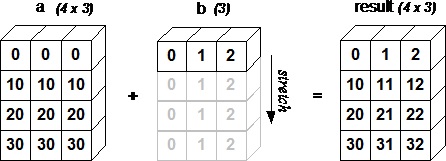

![array](https://www.tutorialspoint.com//numpy/images/array.jpg)

array

数组上的迭代

NumPy 包包含一个迭代器对象numpy.nditer。它是一个有效的多维迭代器对象，可以用于在数组上进行迭代。数组的每个元素可使用 Python 的标准Iterator接口来访问。

让我们使用arange()函数创建一个 3X4 数组，并使用nditer对它进行迭代。

### 示例 1

1. 

   `import numpy as np`

2. 

   `a = np.arange(0,60,5)`

3. 

   `a = a.reshape(3,4)`

4. 

   `print '原始数组是：'`

5. 

   `print a print '\n'`

6. 

   `print '修改后的数组是：'`

7. 

   `for x in np.nditer(a):`

8. 

   `print x,`

9. 

   

输出如下：

1. 

   `原始数组是：`

2. 

   `[[ 0 5 10 15]`

3. 

   `[20 25 30 35]`

4. 

   `[40 45 50 55]]`

5. 

   

6. 

   `修改后的数组是：`

7. 

   `0 5 10 15 20 25 30 35 40 45 50 55`

8. 

   

9. 

   

### 示例 2

迭代的顺序匹配数组的内容布局，而不考虑特定的排序。 这可以通过迭代上述数组的转置来看到。

1. 

   `import numpy as np`

2. 

   `a = np.arange(0,60,5)`

3. 

   `a = a.reshape(3,4)`

4. 

   `print '原始数组是：'`

5. 

   `print a`

6. 

   `print '\n'`

7. 

   `print '原始数组的转置是：'`

8. 

   `b = a.T`

9. 

   `print b`

10. 

    `print '\n'`

11. 

    `print '修改后的数组是：'`

12. 

    `for x in np.nditer(b):`

13. 

    `print x,`

14. 

    

输出如下：

1. 

   `原始数组是：`

2. 

   `[[ 0 5 10 15]`

3. 

   `[20 25 30 35]`

4. 

   `[40 45 50 55]]`

5. 

   

6. 

   `原始数组的转置是：`

7. 

   `[[ 0 20 40]`

8. 

   `[ 5 25 45]`

9. 

   `[10 30 50]`

10. 

    `[15 35 55]]`

11. 

    

12. 

    `修改后的数组是：`

13. 

    `0 5 10 15 20 25 30 35 40 45 50 55`

14. 

    

15. 

    

## 迭代顺序

如果相同元素使用 F 风格顺序存储，则迭代器选择以更有效的方式对数组进行迭代。

### 示例 1

1. 

   `import numpy as np`

2. 

   `a = np.arange(0,60,5)`

3. 

   `a = a.reshape(3,4)`

4. 

   `print '原始数组是：'`

5. 

   `print a print '\n'`

6. 

   `print '原始数组的转置是：'`

7. 

   `b = a.T`

8. 

   `print b`

9. 

   `print '\n'`

10. 

    `print '以 C 风格顺序排序：'`

11. 

    `c = b.copy(order='C')`

12. 

    `print c for x in np.nditer(c):`

13. 

    `print x,`

14. 

    `print '\n'`

15. 

    `print '以 F 风格顺序排序：'`

16. 

    `c = b.copy(order='F')`

17. 

    `print c`

18. 

    `for x in np.nditer(c):`

19. 

    `print x,`

20. 

    

输出如下：

1. 

   `原始数组是：`

2. 

   `[[ 0 5 10 15]`

3. 

   `[20 25 30 35]`

4. 

   `[40 45 50 55]]`

5. 

   

6. 

   `原始数组的转置是：`

7. 

   `[[ 0 20 40]`

8. 

   `[ 5 25 45]`

9. 

   `[10 30 50]`

10. 

    `[15 35 55]]`

11. 

    

12. 

    `以 C 风格顺序排序：`

13. 

    `[[ 0 20 40]`

14. 

    `[ 5 25 45]`

15. 

    `[10 30 50]`

16. 

    `[15 35 55]]`

17. 

    `0 20 40 5 25 45 10 30 50 15 35 55`

18. 

    

19. 

    `以 F 风格顺序排序：`

20. 

    `[[ 0 20 40]`

21. 

    `[ 5 25 45]`

22. 

    `[10 30 50]`

23. 

    `[15 35 55]]`

24. 

    `0 5 10 15 20 25 30 35 40 45 50 55`

25. 

    

26. 

    

### 示例 2

可以通过显式提醒，来强制`nditer`对象使用某种顺序：

1. 

   `import numpy as np`

2. 

   `a = np.arange(0,60,5)`

3. 

   `a = a.reshape(3,4)`

4. 

   `print '原始数组是：'`

5. 

   `print a`

6. 

   `print '\n'`

7. 

   `print '以 C 风格顺序排序：'`

8. 

   `for x in np.nditer(a, order = 'C'):`

9. 

   `print x,`

10. 

    `print '\n'`

11. 

    `print '以 F 风格顺序排序：'`

12. 

    `for x in np.nditer(a, order = 'F'):`

13. 

    `print x,`

14. 

    

输出如下：

1. 

   `原始数组是：`

2. 

   `[[ 0 5 10 15]`

3. 

   `[20 25 30 35]`

4. 

   `[40 45 50 55]]`

5. 

   

6. 

   `以 C 风格顺序排序：`

7. 

   `0 5 10 15 20 25 30 35 40 45 50 55`

8. 

   

9. 

   `以 F 风格顺序排序：`

10. 

    `0 20 40 5 25 45 10 30 50 15 35 55`

11. 

    

12. 

    

## 修改数组的值

`nditer`对象有另一个可选参数`op_flags`。 其默认值为只读，但可以设置为读写或只写模式。 这将允许使用此迭代器修改数组元素。

### 示例

1. 

   `import numpy as np`

2. 

   `a = np.arange(0,60,5)`

3. 

   `a = a.reshape(3,4)`

4. 

   `print '原始数组是：'`

5. 

   `print a`

6. 

   `print '\n'`

7. 

   `for x in np.nditer(a, op_flags=['readwrite']):`

8. 

   `x[...]=2*x`

9. 

   `print '修改后的数组是：'`

10. 

    `print a`

11. 

    

输出如下：

1. 

   `原始数组是：`

2. 

   `[[ 0 5 10 15]`

3. 

   `[20 25 30 35]`

4. 

   `[40 45 50 55]]`

5. 

   

6. 

   `修改后的数组是：`

7. 

   `[[ 0 10 20 30]`

8. 

   `[ 40 50 60 70]`

9. 

   `[ 80 90 100 110]]`

10. 

    

11. 

    

## 外部循环

`nditer`类的构造器拥有`flags`参数，它可以接受下列值：

| 序号 | 参数及描述                                                   |
| ---- | ------------------------------------------------------------ |
| 1.   | `c_index` 可以跟踪 C 顺序的索引                              |
| 2.   | `f_index` 可以跟踪 Fortran 顺序的索引                        |
| 3.   | `multi-index` 每次迭代可以跟踪一种索引类型                   |
| 4.   | `external_loop` 给出的值是具有多个值的一维数组，而不是零维数组 |

### 示例

在下面的示例中，迭代器遍历对应于每列的一维数组。

1. 

   `import numpy as np`

2. 

   `a = np.arange(0,60,5)`

3. 

   `a = a.reshape(3,4)`

4. 

   `print '原始数组是：'`

5. 

   `print a`

6. 

   `print '\n'`

7. 

   `print '修改后的数组是：'`

8. 

   `for x in np.nditer(a, flags = ['external_loop'], order = 'F'):`

9. 

   `print x,`

10. 

    

输出如下：

1. 

   `原始数组是：`

2. 

   `[[ 0 5 10 15]`

3. 

   `[20 25 30 35]`

4. 

   `[40 45 50 55]]`

5. 

   

6. 

   `修改后的数组是：`

7. 

   `[ 0 20 40] [ 5 25 45] [10 30 50] [15 35 55]`

8. 

   

9. 

   

## 广播迭代

如果两个数组是可广播的，`nditer`组合对象能够同时迭代它们。 假设数组`a`具有维度 3X4，并且存在维度为 1X4 的另一个数组`b`，则使用以下类型的迭代器（数组`b`被广播到`a`的大小）。

### 示例

1. 

   `import numpy as np`

2. 

   `a = np.arange(0,60,5)`

3. 

   `a = a.reshape(3,4)`

4. 

   `print '第一个数组：'`

5. 

   `print a`

6. 

   `print '\n'`

7. 

   `print '第二个数组：'`

8. 

   `b = np.array([1, 2, 3, 4], dtype = int)`

9. 

   `print b`

10. 

    `print '\n'`

11. 

    `print '修改后的数组是：'`

12. 

    `for x,y in np.nditer([a,b]):`

13. 

    `print "%d:%d" % (x,y),`

14. 

    

输出如下：

1. 

   `第一个数组：`

2. 

   `[[ 0 5 10 15]`

3. 

   `[20 25 30 35]`

4. 

   `[40 45 50 55]]`

5. 

   

6. 

   `第二个数组：`

7. 

   `[1 2 3 4]`

8. 

   

9. 

   `修改后的数组是：`

10. 

    `0:1 5:2 10:3 15:4 20:1 25:2 30:3 35:4 40:1 45:2 50:3 55:4`

11. 

    

12.

数组操作

NumPy包中有几个例程用于处理ndarray对象中的元素。它们可以分为以下类型：

修改形状

序号	形状及描述
1.	`reshape` 不改变数据的条件下修改形状
2.	`flat` 数组上的一维迭代器
3.	`flatten` 返回折叠为一维的数组副本
4.	`ravel` 返回连续的展开数组

`numpy.reshape`

这个函数在不改变数据的条件下修改形状，它接受如下参数：

numpy.reshape(arr, newshape, order')

其中：

arr：要修改形状的数组
newshape：整数或者整数数组，新的形状应当兼容原有形状
order：'C'为 C 风格顺序，'F'为 F 风格顺序，'A'为保留原顺序。

例子

import numpy as np
a = np.arange(8)
print '原始数组：'
print a
print '\n'
b = a.reshape(4,2)
print '修改后的数组：'
print b

输出如下：

原始数组：
[0 1 2 3 4 5 6 7]
修改后的数组：
[[0 1]
[2 3]
[4 5]
[6 7]]

`numpy.ndarray.flat`

该函数返回数组上的一维迭代器，行为类似 Python 内建的迭代器。

例子

import numpy as np
a = np.arange(8).reshape(2,4)
print '原始数组：'
print a
print '\n'
print '调用 flat 函数之后：'
# 返回展开数组中的下标的对应元素
print a.flat[5]

输出如下：

原始数组：
[[0 1 2 3]
[4 5 6 7]]
调用 flat 函数之后：
5

`numpy.ndarray.flatten`

该函数返回折叠为一维的数组副本，函数接受下列参数：

ndarray.flatten(order)

其中：

order：'C' — 按行，'F' — 按列，'A' — 原顺序，'k' — 元素在内存中的出现顺序。

例子

import numpy as np
a = np.arange(8).reshape(2,4)
print '原数组：'
print a
print '\n'
# default is column-major
print '展开的数组：'
print a.flatten()
print '\n'
print '以 F 风格顺序展开的数组：'
print a.flatten(order = 'F')

输出如下：

原数组：
[[0 1 2 3]
[4 5 6 7]]
展开的数组：
[0 1 2 3 4 5 6 7]
以 F 风格顺序展开的数组：
[0 4 1 5 2 6 3 7]

`numpy.ravel`

这个函数返回展开的一维数组，并且按需生成副本。返回的数组和输入数组拥有相同数据类型。这个函数接受两个参数。

numpy.ravel(a, order)

构造器接受下列参数：

order：'C' — 按行，'F' — 按列，'A' — 原顺序，'k' — 元素在内存中的出现顺序。

例子

import numpy as np
a = np.arange(8).reshape(2,4)
print '原数组：'
print a
print '\n'
print '调用 ravel 函数之后：'
print a.ravel()
print '\n'
print '以 F 风格顺序调用 ravel 函数之后：'
print a.ravel(order = 'F')
原数组：
[[0 1 2 3]
[4 5 6 7]]
调用 ravel 函数之后：
[0 1 2 3 4 5 6 7]
以 F 风格顺序调用 ravel 函数之后：
[0 4 1 5 2 6 3 7]

翻转操作

序号	操作及描述
1.	`transpose` 翻转数组的维度
2.	`ndarray.T` 和`self.transpose()`相同
3.	`rollaxis` 向后滚动指定的轴
4.	`swapaxes` 互换数组的两个轴

`numpy.transpose`

这个函数翻转给定数组的维度。如果可能的话它会返回一个视图。函数接受下列参数：

numpy.transpose(arr, axes)

其中：

arr：要转置的数组
axes：整数的列表，对应维度，通常所有维度都会翻转。

例子

import numpy as np
a = np.arange(12).reshape(3,4)
print '原数组：'
print a
print '\n'
print '转置数组：'
print np.transpose(a)

输出如下：

原数组：
[[ 0 1 2 3]
[ 4 5 6 7]
[ 8 9 10 11]]
转置数组：
[[ 0 4 8]
[ 1 5 9]
[ 2 6 10]
[ 3 7 11]]

`numpy.ndarray.T`

该函数属于ndarray类，行为类似于numpy.transpose。

例子

import numpy as np
a = np.arange(12).reshape(3,4)
print '原数组：'
print a
print '\n'
print '转置数组：'
print a.T

输出如下：

原数组：
[[ 0 1 2 3]
[ 4 5 6 7]
[ 8 9 10 11]]
转置数组：
[[ 0 4 8]
[ 1 5 9]
[ 2 6 10]
[ 3 7 11]]

`numpy.rollaxis`

该函数向后滚动特定的轴，直到一个特定位置。这个函数接受三个参数：

numpy.rollaxis(arr, axis, start)

其中：

arr：输入数组
axis：要向后滚动的轴，其它轴的相对位置不会改变
start：默认为零，表示完整的滚动。会滚动到特定位置。

例子

# 创建了三维的 ndarray
import numpy as np
a = np.arange(8).reshape(2,2,2)
print '原数组：'
print a
print '\n'
# 将轴 2 滚动到轴 0（宽度到深度）
print '调用 rollaxis 函数：'
print np.rollaxis(a,2)
# 将轴 0 滚动到轴 1：（宽度到高度）
print '\n'
print '调用 rollaxis 函数：'
print np.rollaxis(a,2,1)

输出如下：

原数组：
[[[0 1]
[2 3]]
[[4 5]
[6 7]]]
调用 rollaxis 函数：
[[[0 2]
[4 6]]
[[1 3]
[5 7]]]
调用 rollaxis 函数：
[[[0 2]
[1 3]]
[[4 6]
[5 7]]]

`numpy.swapaxes`

该函数交换数组的两个轴。对于 1.10 之前的 NumPy 版本，会返回交换后数组的试图。这个函数接受下列参数：

numpy.swapaxes(arr, axis1, axis2)

arr：要交换其轴的输入数组
axis1：对应第一个轴的整数
axis2：对应第二个轴的整数

# 创建了三维的 ndarray
import numpy as np
a = np.arange(8).reshape(2,2,2)
print '原数组：'
print a
print '\n'
# 现在交换轴 0（深度方向）到轴 2（宽度方向）
print '调用 swapaxes 函数后的数组：'
print np.swapaxes(a, 2, 0)

输出如下：

原数组：
[[[0 1]
[2 3]]
[[4 5]
[6 7]]]
调用 swapaxes 函数后的数组：
[[[0 4]
[2 6]]
[[1 5]
[3 7]]]

修改维度

序号	维度和描述
1.	`broadcast` 产生模仿广播的对象
2.	`broadcast_to` 将数组广播到新形状
3.	`expand_dims` 扩展数组的形状
4.	`squeeze` 从数组的形状中删除单维条目

`broadcast`

如前所述，NumPy 已经内置了对广播的支持。此功能模仿广播机制。它返回一个对象，该对象封装了将一个数组广播到另一个数组的结果。

该函数使用两个数组作为输入参数。下面的例子说明了它的用法。

import numpy as np
x = np.array([[1], [2], [3]])
y = np.array([4, 5, 6])
# 对 y 广播 x
b = np.broadcast(x,y)
# 它拥有 iterator 属性，基于自身组件的迭代器元组
print '对 y 广播 x：'
r,c = b.iters
print r.next(), c.next()
print r.next(), c.next()
print '\n'
# shape 属性返回广播对象的形状
print '广播对象的形状：'
print b.shape
print '\n'
# 手动使用 broadcast 将 x 与 y 相加
b = np.broadcast(x,y)
c = np.empty(b.shape)
print '手动使用 broadcast 将 x 与 y 相加：'
print c.shape
print '\n'
c.flat = [u + v for (u,v) in b]
print '调用 flat 函数：'
print c
print '\n'
# 获得了和 NumPy 内建的广播支持相同的结果
print 'x 与 y 的和：'
print x + y

输出如下：

对 y 广播 x：
1 4
1 5
广播对象的形状：
(3, 3)
手动使用 broadcast 将 x 与 y 相加：
(3, 3)
调用 flat 函数：
[[ 5. 6. 7.]
[ 6. 7. 8.]
[ 7. 8. 9.]]
x 与 y 的和：
[[5 6 7]
[6 7 8]
[7 8 9]]

`numpy.broadcast_to`

此函数将数组广播到新形状。它在原始数组上返回只读视图。它通常不连续。如果新形状不符合 NumPy 的广播规则，该函数可能会抛出ValueError。

注意 – 此功能可用于 1.10.0 及以后的版本。

该函数接受以下参数。

numpy.broadcast_to(array, shape, subok)

例子

import numpy as np
a = np.arange(4).reshape(1,4)
print '原数组：'
print a
print '\n'
print '调用 broadcast_to 函数之后：'
print np.broadcast_to(a,(4,4))

输出如下：

[[0 1 2 3]
[0 1 2 3]
[0 1 2 3]
[0 1 2 3]]

`numpy.expand_dims`

函数通过在指定位置插入新的轴来扩展数组形状。该函数需要两个参数：

numpy.expand_dims(arr, axis)

其中：

arr：输入数组
axis：新轴插入的位置

例子

import numpy as np
x = np.array(([1,2],[3,4]))
print '数组 x：'
print x
print '\n'
y = np.expand_dims(x, axis = 0)
print '数组 y：'
print y
print '\n'
print '数组 x 和 y 的形状：'
print x.shape, y.shape
print '\n'
# 在位置 1 插入轴
y = np.expand_dims(x, axis = 1)
print '在位置 1 插入轴之后的数组 y：'
print y
print '\n'
print 'x.ndim 和 y.ndim：'
print x.ndim,y.ndim
print '\n'
print 'x.shape 和 y.shape：'
print x.shape, y.shape

输出如下：

数组 x：
[[1 2]
[3 4]]
数组 y：
[[[1 2]
[3 4]]]
数组 x 和 y 的形状：
(2, 2) (1, 2, 2)
在位置 1 插入轴之后的数组 y：
[[[1 2]]
[[3 4]]]
x.shape 和 y.shape：
2 3
x.shape and y.shape:
(2, 2) (2, 1, 2)

`numpy.squeeze`

函数从给定数组的形状中删除一维条目。此函数需要两个参数。

numpy.squeeze(arr, axis)

其中：

arr：输入数组
axis：整数或整数元组，用于选择形状中单一维度条目的子集

例子

import numpy as np
x = np.arange(9).reshape(1,3,3)
print '数组 x：'
print x
print '\n'
y = np.squeeze(x)
print '数组 y：'
print y
print '\n'
print '数组 x 和 y 的形状：'
print x.shape, y.shape

输出如下：

数组 x：
[[[0 1 2]
[3 4 5]
[6 7 8]]]
数组 y：
[[0 1 2]
[3 4 5]
[6 7 8]]
数组 x 和 y 的形状：
(1, 3, 3) (3, 3)

数组的连接

序号	数组及描述
1.	`concatenate` 沿着现存的轴连接数据序列
2.	`stack` 沿着新轴连接数组序列
3.	`hstack` 水平堆叠序列中的数组（列方向）
4.	`vstack` 竖直堆叠序列中的数组（行方向）

`numpy.concatenate`

数组的连接是指连接。此函数用于沿指定轴连接相同形状的两个或多个数组。该函数接受以下参数。

numpy.concatenate((a1, a2, ...), axis)

其中：

a1, a2, ...：相同类型的数组序列
axis：沿着它连接数组的轴，默认为 0

例子

import numpy as np
a = np.array([[1,2],[3,4]])
print '第一个数组：'
print a
print '\n'
b = np.array([[5,6],[7,8]])
print '第二个数组：'
print b
print '\n'
# 两个数组的维度相同
print '沿轴 0 连接两个数组：'
print np.concatenate((a,b))
print '\n'
print '沿轴 1 连接两个数组：'
print np.concatenate((a,b),axis = 1)

输出如下：

第一个数组：
[[1 2]
[3 4]]
第二个数组：
[[5 6]
[7 8]]
沿轴 0 连接两个数组：
[[1 2]
[3 4]
[5 6]
[7 8]]
沿轴 1 连接两个数组：
[[1 2 5 6]
[3 4 7 8]]

`numpy.stack`

此函数沿新轴连接数组序列。此功能添加自 NumPy 版本 1.10.0。需要提供以下参数。

numpy.stack(arrays, axis)

其中：

arrays：相同形状的数组序列
axis：返回数组中的轴，输入数组沿着它来堆叠

import numpy as np
a = np.array([[1,2],[3,4]])
print '第一个数组：'
print a
print '\n'
b = np.array([[5,6],[7,8]])
print '第二个数组：'
print b
print '\n'
print '沿轴 0 堆叠两个数组：'
print np.stack((a,b),0)
print '\n'
print '沿轴 1 堆叠两个数组：'
print np.stack((a,b),1)

输出如下：

第一个数组：
[[1 2]
[3 4]]
第二个数组：
[[5 6]
[7 8]]
沿轴 0 堆叠两个数组：
[[[1 2]
[3 4]]
[[5 6]
[7 8]]]
沿轴 1 堆叠两个数组：
[[[1 2]
[5 6]]
[[3 4]
[7 8]]]

`numpy.hstack`

numpy.stack函数的变体，通过堆叠来生成水平的单个数组。

例子

import numpy as np
a = np.array([[1,2],[3,4]])
print '第一个数组：'
print a
print '\n'
b = np.array([[5,6],[7,8]])
print '第二个数组：'
print b
print '\n'
print '水平堆叠：'
c = np.hstack((a,b))
print c
print '\n'

输出如下：

第一个数组：
[[1 2]
[3 4]]
第二个数组：
[[5 6]
[7 8]]
水平堆叠：
[[1 2 5 6]
[3 4 7 8]]

`numpy.vstack`

numpy.stack函数的变体，通过堆叠来生成竖直的单个数组。

import numpy as np
a = np.array([[1,2],[3,4]])
print '第一个数组：'
print a
print '\n'
b = np.array([[5,6],[7,8]])
print '第二个数组：'
print b
print '\n'
print '竖直堆叠：'
c = np.vstack((a,b))
print c

输出如下：

第一个数组：
[[1 2]
[3 4]]
第二个数组：
[[5 6]
[7 8]]
竖直堆叠：
[[1 2]
[3 4]
[5 6]
[7 8]]

数组分割

序号	数组及操作
1.	`split` 将一个数组分割为多个子数组
2.	`hsplit` 将一个数组水平分割为多个子数组（按列）
3.	`vsplit` 将一个数组竖直分割为多个子数组（按行）

`numpy.split`

该函数沿特定的轴将数组分割为子数组。函数接受三个参数：

numpy.split(ary, indices_or_sections, axis)

其中：

ary：被分割的输入数组
indices_or_sections：可以是整数，表明要从输入数组创建的，等大小的子数组的数量。如果此参数是一维数组，则其元素表明要创建新子数组的点。
axis：默认为 0

例子

import numpy as np
a = np.arange(9)
print '第一个数组：'
print a
print '\n'
print '将数组分为三个大小相等的子数组：'
b = np.split(a,3)
print b
print '\n'
print '将数组在一维数组中表明的位置分割：'
b = np.split(a,[4,7])
print b

输出如下：

第一个数组：
[0 1 2 3 4 5 6 7 8]
将数组分为三个大小相等的子数组：
[array([0, 1, 2]), array([3, 4, 5]), array([6, 7, 8])]
将数组在一维数组中表明的位置分割：
[array([0, 1, 2, 3]), array([4, 5, 6]), array([7, 8])]

`numpy.hsplit`

numpy.hsplit是split()函数的特例，其中轴为 1 表示水平分割，无论输入数组的维度是什么。

import numpy as np
a = np.arange(16).reshape(4,4)
print '第一个数组：'
print a
print '\n'
print '水平分割：'
b = np.hsplit(a,2)
print b
print '\n'

输出：

第一个数组：
[[ 0 1 2 3]
[ 4 5 6 7]
[ 8 9 10 11]
[12 13 14 15]]
水平分割：
[array([[ 0, 1],
[ 4, 5],
[ 8, 9],
[12, 13]]), array([[ 2, 3],
[ 6, 7],
[10, 11],
[14, 15]])]

`numpy.vsplit`

numpy.vsplit是split()函数的特例，其中轴为 0 表示竖直分割，无论输入数组的维度是什么。下面的例子使之更清楚。

import numpy as np
a = np.arange(16).reshape(4,4)
print '第一个数组：'
print a
print '\n'
print '竖直分割：'
b = np.vsplit(a,2)
print b

输出如下：

第一个数组：
[[ 0 1 2 3]
[ 4 5 6 7]
[ 8 9 10 11]
[12 13 14 15]]
竖直分割：
[array([[0, 1, 2, 3],
[4, 5, 6, 7]]), array([[ 8, 9, 10, 11],
[12, 13, 14, 15]])]

添加/删除元素

序号	元素及描述
1.	`resize` 返回指定形状的新数组
2.	`append` 将值添加到数组末尾
3.	`insert` 沿指定轴将值插入到指定下标之前
4.	`delete` 返回删掉某个轴的子数组的新数组
5.	`unique` 寻找数组内的唯一元素

`numpy.resize`

此函数返回指定大小的新数组。如果新大小大于原始大小，则包含原始数组中的元素的重复副本。该函数接受以下参数。

numpy.resize(arr, shape)

其中：

arr：要修改大小的输入数组
shape：返回数组的新形状

例子

import numpy as np
a = np.array([[1,2,3],[4,5,6]])
print '第一个数组：'
print a
print '\n'
print '第一个数组的形状：'
print a.shape
print '\n'
b = np.resize(a, (3,2))
print '第二个数组：'
print b
print '\n'
print '第二个数组的形状：'
print b.shape
print '\n'
# 要注意 a 的第一行在 b 中重复出现，因为尺寸变大了
print '修改第二个数组的大小：'
b = np.resize(a,(3,3))
print b

输出如下：

第一个数组：
[[1 2 3]
[4 5 6]]
第一个数组的形状：
(2, 3)
第二个数组：
[[1 2]
[3 4]
[5 6]]
第二个数组的形状：
(3, 2)
修改第二个数组的大小：
[[1 2 3]
[4 5 6]
[1 2 3]]

`numpy.append`

此函数在输入数组的末尾添加值。附加操作不是原地的，而是分配新的数组。此外，输入数组的维度必须匹配否则将生成ValueError。

函数接受下列函数：

numpy.append(arr, values, axis)

其中：

arr：输入数组
values：要向arr添加的值，比如和arr形状相同（除了要添加的轴）
axis：沿着它完成操作的轴。如果没有提供，两个参数都会被展开。

例子

import numpy as np
a = np.array([[1,2,3],[4,5,6]])
print '第一个数组：'
print a
print '\n'
print '向数组添加元素：'
print np.append(a, [7,8,9])
print '\n'
print '沿轴 0 添加元素：'
print np.append(a, [[7,8,9]],axis = 0)
print '\n'
print '沿轴 1 添加元素：'
print np.append(a, [[5,5,5],[7,8,9]],axis = 1)

输出如下：

第一个数组：
[[1 2 3]
[4 5 6]]
向数组添加元素：
[1 2 3 4 5 6 7 8 9]
沿轴 0 添加元素：
[[1 2 3]
[4 5 6]
[7 8 9]]
沿轴 1 添加元素：
[[1 2 3 5 5 5]
[4 5 6 7 8 9]]

`numpy.insert`

此函数在给定索引之前，沿给定轴在输入数组中插入值。如果值的类型转换为要插入，则它与输入数组不同。插入没有原地的，函数会返回一个新数组。此外，如果未提供轴，则输入数组会被展开。

insert()函数接受以下参数：

numpy.insert(arr, obj, values, axis)

其中：

arr：输入数组
obj：在其之前插入值的索引
values：要插入的值
axis：沿着它插入的轴，如果未提供，则输入数组会被展开

例子

import numpy as np
a = np.array([[1,2],[3,4],[5,6]])
print '第一个数组：'
print a
print '\n'
print '未传递 Axis 参数。在插入之前输入数组会被展开。'
print np.insert(a,3,[11,12])
print '\n'
print '传递了 Axis 参数。会广播值数组来配输入数组。'
print '沿轴 0 广播：'
print np.insert(a,1,[11],axis = 0)
print '\n'
print '沿轴 1 广播：'
print np.insert(a,1,11,axis = 1)

`numpy.delete`

此函数返回从输入数组中删除指定子数组的新数组。与insert()函数的情况一样，如果未提供轴参数，则输入数组将展开。该函数接受以下参数：

Numpy.delete(arr, obj, axis)

其中：

arr：输入数组
obj：可以被切片，整数或者整数数组，表明要从输入数组删除的子数组
axis：沿着它删除给定子数组的轴，如果未提供，则输入数组会被展开

例子

import numpy as np
a = np.arange(12).reshape(3,4)
print '第一个数组：'
print a
print '\n'
print '未传递 Axis 参数。在插入之前输入数组会被展开。'
print np.delete(a,5)
print '\n'
print '删除第二列：'
print np.delete(a,1,axis = 1)
print '\n'
print '包含从数组中删除的替代值的切片：'
a = np.array([1,2,3,4,5,6,7,8,9,10])
print np.delete(a, np.s_[::2])

输出如下：

第一个数组：
[[ 0 1 2 3]
[ 4 5 6 7]
[ 8 9 10 11]]
未传递 Axis 参数。在插入之前输入数组会被展开。
[ 0 1 2 3 4 6 7 8 9 10 11]
删除第二列：
[[ 0 2 3]
[ 4 6 7]
[ 8 10 11]]
包含从数组中删除的替代值的切片：
[ 2 4 6 8 10]

`numpy.unique`

此函数返回输入数组中的去重元素数组。该函数能够返回一个元组，包含去重数组和相关索引的数组。索引的性质取决于函数调用中返回参数的类型。

numpy.unique(arr, return_index, return_inverse, return_counts)

其中：

arr：输入数组，如果不是一维数组则会展开
return_index：如果为true，返回输入数组中的元素下标
return_inverse：如果为true，返回去重数组的下标，它可以用于重构输入数组
return_counts：如果为true，返回去重数组中的元素在原数组中的出现次数

例子

import numpy as np
a = np.array([5,2,6,2,7,5,6,8,2,9])
print '第一个数组：'
print a
print '\n'
print '第一个数组的去重值：'
u = np.unique(a)
print u
print '\n'
print '去重数组的索引数组：'
u,indices = np.unique(a, return_index = True)
print indices
print '\n'
print '我们可以看到每个和原数组下标对应的数值：'
print a
print '\n'
print '去重数组的下标：'
u,indices = np.unique(a,return_inverse = True)
print u
print '\n'
print '下标为：'
print indices
print '\n'
print '使用下标重构原数组：'
print u[indices]
print '\n'
print '返回去重元素的重复数量：'
u,indices = np.unique(a,return_counts = True)
print u
print indices

输出如下：

第一个数组：
[5 2 6 2 7 5 6 8 2 9]
第一个数组的去重值：
[2 5 6 7 8 9]
去重数组的索引数组：
[1 0 2 4 7 9]
我们可以看到每个和原数组下标对应的数值：
[5 2 6 2 7 5 6 8 2 9]
去重数组的下标：
[2 5 6 7 8 9]
下标为：
[1 0 2 0 3 1 2 4 0 5]
使用下标重构原数组：
[5 2 6 2 7 5 6 8 2 9]
返回唯一元素的重复数量：
[2 5 6 7 8 9]
[3 2 2 1 1 1]

NumPy – 位操作

下面是 NumPy 包中可用的位操作函数。

序号	操作及描述
1.	`bitwise_and` 对数组元素执行位与操作
2.	`bitwise_or` 对数组元素执行位或操作
3.	`invert` 计算位非
4.	`left_shift` 向左移动二进制表示的位
5.	`right_shift` 向右移动二进制表示的位

`bitwise_and`

通过np.bitwise_and()函数对输入数组中的整数的二进制表示的相应位执行位与运算。

例子

import numpy as np
print '13 和 17 的二进制形式：'
a,b = 13,17
print bin(a), bin(b)
print '\n'
print '13 和 17 的位与：'
print np.bitwise_and(13, 17)

输出如下：

13 和 17 的二进制形式：
0b1101 0b10001
13 和 17 的位与：
1

你可以使用下表验证此输出。考虑下面的位与真值表。

A	B	AND
1	1	1
1	0	0
0	1	0
0	0	0

		1	1	0	1
AND
	1	0	0	0	1
result	0	0	0	0	1

`bitwise_or`

通过np.bitwise_or()函数对输入数组中的整数的二进制表示的相应位执行位或运算。

例子

import numpy as np
a,b = 13,17
print '13 和 17 的二进制形式：'
print bin(a), bin(b)
print '13 和 17 的位或：'
print np.bitwise_or(13, 17)

输出如下：

13 和 17 的二进制形式：
0b1101 0b10001
13 和 17 的位或：
29

你可以使用下表验证此输出。考虑下面的位或真值表。

A	B	OR
1	1	1
1	0	1
0	1	1
0	0	0

		1	1	0	1
OR
	1	0	0	0	1
result	1	1	1	0	1

`invert`

此函数计算输入数组中整数的位非结果。对于有符号整数，返回补码。

例子

import numpy as np
print '13 的位反转，其中 ndarray 的 dtype 是 uint8：'
print np.invert(np.array([13], dtype = np.uint8))
print '\n'
# 比较 13 和 242 的二进制表示，我们发现了位的反转
print '13 的二进制表示：'
print np.binary_repr(13, width = 8)
print '\n'
print '242 的二进制表示：'
print np.binary_repr(242, width = 8)

输出如下：

13 的位反转，其中 ndarray 的 dtype 是 uint8：
[242]
13 的二进制表示：
00001101
242 的二进制表示：
11110010

请注意，np.binary_repr()函数返回给定宽度中十进制数的二进制表示。

`left_shift`

numpy.left shift()函数将数组元素的二进制表示中的位向左移动到指定位置，右侧附加相等数量的 0。

例如，

import numpy as np
print '将 10 左移两位：'
print np.left_shift(10,2)
print '\n'
print '10 的二进制表示：'
print np.binary_repr(10, width = 8)
print '\n'
print '40 的二进制表示：'
print np.binary_repr(40, width = 8)
# '00001010' 中的两位移动到了左边，并在右边添加了两个 0。

输出如下：

将 10 左移两位：
40
10 的二进制表示：
00001010
40 的二进制表示：
00101000

`right_shift`

numpy.right_shift()函数将数组元素的二进制表示中的位向右移动到指定位置，左侧附加相等数量的 0。

import numpy as np
print '将 40 右移两位：'
print np.right_shift(40,2)
print '\n'
print '40 的二进制表示：'
print np.binary_repr(40, width = 8)
print '\n'
print '10 的二进制表示：'
print np.binary_repr(10, width = 8)
# '00001010' 中的两位移动到了右边，并在左边添加了两个 0。

输出如下：

将 40 右移两位：
10
40 的二进制表示：
00101000
10 的二进制表示：
00001010

NumPy – 字符串函数

以下函数用于对dtype为numpy.string_或numpy.unicode_的数组执行向量化字符串操作。它们基于 Python 内置库中的标准字符串函数。

序号	函数及描述
1.	`add()` 返回两个`str`或`Unicode`数组的逐个字符串连接
2.	`multiply()` 返回按元素多重连接后的字符串
3.	`center()` 返回给定字符串的副本，其中元素位于特定字符串的中央
4.	`capitalize()` 返回给定字符串的副本，其中只有第一个字符串大写
5.	`title()` 返回字符串或 Unicode 的按元素标题转换版本
6.	`lower()` 返回一个数组，其元素转换为小写
7.	`upper()` 返回一个数组，其元素转换为大写
8.	`split()` 返回字符串中的单词列表，并使用分隔符来分割
9.	`splitlines()` 返回元素中的行列表，以换行符分割
10.	`strip()` 返回数组副本，其中元素移除了开头或者结尾处的特定字符
11.	`join()` 返回一个字符串，它是序列中字符串的连接
12.	`replace()` 返回字符串的副本，其中所有子字符串的出现位置都被新字符串取代
13.	`decode()` 按元素调用`str.decode`
14.	`encode()` 按元素调用`str.encode`

这些函数在字符数组类（numpy.char）中定义。较旧的 Numarray 包包含chararray类。 numpy.char类中的上述函数在执行向量化字符串操作时非常有用。

`numpy.char.add()`

函数执行按元素的字符串连接。

import numpy as np
print '连接两个字符串：'
print np.char.add(['hello'],[' xyz'])
print '\n'
print '连接示例：'
print np.char.add(['hello', 'hi'],[' abc', ' xyz'])

输出如下：

连接两个字符串：
[‘hello xyz’]
连接示例：
[‘hello abc’ ‘hi xyz’]

`numpy.char.multiply()`

这个函数执行多重连接。

import numpy as np
print np.char.multiply('Hello ',3)

输出如下：

Hello Hello Hello

`numpy.char.center()`

此函数返回所需宽度的数组，以便输入字符串位于中心，并使用fillchar在左侧和右侧进行填充。

import numpy as np
# np.char.center(arr, width,fillchar)
print np.char.center('hello', 20,fillchar = '*')

输出如下：

*******hello********

`numpy.char.capitalize()`

函数返回字符串的副本，其中第一个字母大写

import numpy as np
print np.char.capitalize('hello world')

输出如下：

Hello world

`numpy.char.title()`

返回输入字符串的按元素标题转换版本，其中每个单词的首字母都大写。

import numpy as np
print np.char.title('hello how are you?')

输出如下：

Hello How Are You?

`numpy.char.lower()`

函数返回一个数组，其元素转换为小写。它对每个元素调用str.lower。

import numpy as np
print np.char.lower(['HELLO','WORLD'])
print np.char.lower('HELLO')

输出如下：

[‘hello’ ‘world’]
hello

`numpy.char.upper()`

函数返回一个数组，其元素转换为大写。它对每个元素调用str.upper。

import numpy as np
print np.char.upper('hello')
print np.char.upper(['hello','world'])

输出如下：

HELLO
[‘HELLO’ ‘WORLD’]

`numpy.char.split()`

此函数返回输入字符串中的单词列表。默认情况下，空格用作分隔符。否则，指定的分隔符字符用于分割字符串。

import numpy as np
print np.char.split ('hello how are you?')
print np.char.split ('TutorialsPoint,Hyderabad,Telangana', sep = ',')

输出如下：

[‘hello’, ‘how’, ‘are’, ‘you?’]
[‘TutorialsPoint’, ‘Hyderabad’, ‘Telangana’]

`numpy.char.splitlines()`

函数返回数组中元素的单词列表，以换行符分割。

import numpy as np
print np.char.splitlines('hello\nhow are you?')
print np.char.splitlines('hello\rhow are you?')

输出如下：

[‘hello’, ‘how are you?’]
[‘hello’, ‘how are you?’]

'\n'，'\r'，'\r\n'都会用作换行符。

`numpy.char.strip()`

函数返回数组的副本，其中元素移除了开头或结尾处的特定字符。

import numpy as np
print np.char.strip('ashok arora','a')
print np.char.strip(['arora','admin','java'],'a')

输出如下：

shok aror
[‘ror’ ‘dmin’ ‘jav’]

`numpy.char.join()`

这个函数返回一个字符串，其中单个字符由特定的分隔符连接。

import numpy as np
print np.char.join(':','dmy')
print np.char.join([':','-'],['dmy','ymd'])

输出如下：

d:m:y
['d:m:y' 'y-m-d']

`numpy.char.replace()`

这个函数返回字符串副本，其中所有字符序列的出现位置都被另一个给定的字符序列取代。

import numpy as np
print np.char.replace ('He is a good boy', 'is', 'was')

输出如下：

He was a good boy

`numpy.char.decode()`

这个函数在给定的字符串中使用特定编码调用str.decode()。

import numpy as np
a = np.char.encode('hello', 'cp500')
print a
print np.char.decode(a,'cp500')

输出如下：

\x88\x85\x93\x93\x96
hello

`numpy.char.encode()`

此函数对数组中的每个元素调用str.encode函数。默认编码是utf_8，可以使用标准 Python 库中的编解码器。

import numpy as np
a = np.char.encode('hello', 'cp500')
print a

输出如下：

\x88\x85\x93\x93\x96

NumPy – 算数函数

很容易理解的是，NumPy 包含大量的各种数学运算功能。 NumPy 提供标准的三角函数，算术运算的函数，复数处理函数等。

三角函数

NumPy 拥有标准的三角函数，它为弧度制单位的给定角度返回三角函数比值。

示例

import numpy as np
a = np.array([0,30,45,60,90])
print '不同角度的正弦值：'
# 通过乘 pi/180 转化为弧度
print np.sin(a*np.pi/180)
print '\n'
print '数组中角度的余弦值：'
print np.cos(a*np.pi/180)
print '\n'
print '数组中角度的正切值：'
print np.tan(a*np.pi/180)

输出如下：

不同角度的正弦值：
[ 0. 0.5 0.70710678 0.8660254 1. ]
数组中角度的余弦值：
[ 1.00000000e+00 8.66025404e-01 7.07106781e-01 5.00000000e-01
6.12323400e-17]
数组中角度的正切值：
[ 0.00000000e+00 5.77350269e-01 1.00000000e+00 1.73205081e+00
1.63312394e+16]

arcsin，arccos，和arctan函数返回给定角度的sin，cos和tan的反三角函数。这些函数的结果可以通过numpy.degrees()函数通过将弧度制转换为角度制来验证。

示例

import numpy as np
a = np.array([0,30,45,60,90])
print '含有正弦值的数组：'
sin = np.sin(a*np.pi/180)
print sin
print '\n'
print '计算角度的反正弦，返回值以弧度为单位：'
inv = np.arcsin(sin)
print inv
print '\n'
print '通过转化为角度制来检查结果：'
print np.degrees(inv)
print '\n'
print 'arccos 和 arctan 函数行为类似：'
cos = np.cos(a*np.pi/180)
print cos
print '\n'
print '反余弦：'
inv = np.arccos(cos)
print inv
print '\n'
print '角度制单位：'
print np.degrees(inv)
print '\n'
print 'tan 函数：'
tan = np.tan(a*np.pi/180)
print tan
print '\n'
print '反正切：'
inv = np.arctan(tan)
print inv
print '\n'
print '角度制单位：'
print np.degrees(inv)

输出如下：

含有正弦值的数组：
[ 0. 0.5 0.70710678 0.8660254 1. ]
计算角度的反正弦，返回值以弧度制为单位：
[ 0. 0.52359878 0.78539816 1.04719755 1.57079633]
通过转化为角度制来检查结果：
[ 0. 30. 45. 60. 90.]
arccos 和 arctan 函数行为类似：
[ 1.00000000e+00 8.66025404e-01 7.07106781e-01 5.00000000e-01
6.12323400e-17]
反余弦：
[ 0. 0.52359878 0.78539816 1.04719755 1.57079633]
角度制单位：
[ 0. 30. 45. 60. 90.]
tan 函数：
[ 0.00000000e+00 5.77350269e-01 1.00000000e+00 1.73205081e+00
1.63312394e+16]
反正切：
[ 0. 0.52359878 0.78539816 1.04719755 1.57079633]
角度制单位：
[ 0. 30. 45. 60. 90.]

舍入函数

`numpy.around()`

这个函数返回四舍五入到所需精度的值。该函数接受以下参数。

numpy.around(a,decimals)

其中：

序号	参数及描述
1.	`a` 输入数组
2.	`decimals` 要舍入的小数位数。默认值为0。如果为负，整数将四舍五入到小数点左侧的位置

示例

import numpy as np
a = np.array([1.0,5.55, 123, 0.567, 25.532])
print '原数组：'
print a
print '\n'
print '舍入后：'
print np.around(a)
print np.around(a, decimals = 1)
print np.around(a, decimals = -1)

输出如下：

原数组：
[ 1. 5.55 123. 0.567 25.532]
舍入后：
[ 1. 6. 123. 1. 26. ]
[ 1. 5.6 123. 0.6 25.5]
[ 0. 10. 120. 0. 30. ]

`numpy.floor()`

此函数返回不大于输入参数的最大整数。即标量x 的下限是最大的整数i ，使得i <= x。注意在Python中，向下取整总是从 0 舍入。

示例

import numpy as np
a = np.array([-1.7, 1.5, -0.2, 0.6, 10])
print '提供的数组：'
print a
print '\n'
print '修改后的数组：'
print np.floor(a)

输出如下：

提供的数组：
[ -1.7 1.5 -0.2 0.6 10. ]
修改后的数组：
[ -2. 1. -1. 0. 10.]

`numpy.ceil()`

ceil()函数返回输入值的上限，即，标量x的上限是最小的整数i ，使得i> = x。

示例

import numpy as np
a = np.array([-1.7, 1.5, -0.2, 0.6, 10])
print '提供的数组：'
print a
print '\n'
print '修改后的数组：'
print np.ceil(a)

输出如下：

提供的数组：
[ -1.7 1.5 -0.2 0.6 10. ]
修改后的数组：
[ -1. 2. -0. 1. 10.]

NumPy – 算数运算

用于执行算术运算（如add()，subtract()，multiply()和divide()）的输入数组必须具有相同的形状或符合数组广播规则。

示例

import numpy as np
a = np.arange(9, dtype = np.float_).reshape(3,3)
print '第一个数组：'
print a
print '\n'
print '第二个数组：'
b = np.array([10,10,10])
print b
print '\n'
print '两个数组相加：'
print np.add(a,b)
print '\n'
print '两个数组相减：'
print np.subtract(a,b)
print '\n'
print '两个数组相乘：'
print np.multiply(a,b)
print '\n'
print '两个数组相除：'
print np.divide(a,b)

输出如下：

第一个数组：
[[ 0. 1. 2.]
[ 3. 4. 5.]
[ 6. 7. 8.]]
第二个数组：
[10 10 10]
两个数组相加：
[[ 10. 11. 12.]
[ 13. 14. 15.]
[ 16. 17. 18.]]
两个数组相减：
[[-10. -9. -8.]
[ -7. -6. -5.]
[ -4. -3. -2.]]
两个数组相乘：
[[ 0. 10. 20.]
[ 30. 40. 50.]
[ 60. 70. 80.]]
两个数组相除：
[[ 0. 0.1 0.2]
[ 0.3 0.4 0.5]
[ 0.6 0.7 0.8]]

让我们现在来讨论 NumPy 中提供的一些其他重要的算术函数。

`numpy.reciprocal()`

此函数返回参数逐元素的倒数，。由于 Python 处理整数除法的方式，对于绝对值大于 1 的整数元素，结果始终为 0，对于整数 0，则发出溢出警告。

示例

import numpy as np
a = np.array([0.25, 1.33, 1, 0, 100])
print '我们的数组是：'
print a
print '\n'
print '调用 reciprocal 函数：'
print np.reciprocal(a)
print '\n'
b = np.array([100], dtype = int)
print '第二个数组：'
print b
print '\n'
print '调用 reciprocal 函数：'
print np.reciprocal(b)

输出如下：

我们的数组是：
[ 0.25 1.33 1. 0. 100. ]
调用 reciprocal 函数：
main.py:9: RuntimeWarning: divide by zero encountered in reciprocal
print np.reciprocal(a)
[ 4. 0.7518797 1. inf 0.01 ]
第二个数组：
[100]
调用 reciprocal 函数：
[0]

`numpy.power()`

此函数将第一个输入数组中的元素作为底数，计算它与第二个输入数组中相应元素的幂。

import numpy as np
a = np.array([10,100,1000])
print '我们的数组是；'
print a
print '\n'
print '调用 power 函数：'
print np.power(a,2)
print '\n'
print '第二个数组：'
b = np.array([1,2,3])
print b
print '\n'
print '再次调用 power 函数：'
print np.power(a,b)

输出如下：

我们的数组是；
[ 10 100 1000]
调用 power 函数：
[ 100 10000 1000000]
第二个数组：
[1 2 3]
再次调用 power 函数：
[ 10 10000 1000000000]

`numpy.mod()`

此函数返回输入数组中相应元素的除法余数。函数numpy.remainder()也产生相同的结果。

import numpy as np
a = np.array([10,20,30])
b = np.array([3,5,7])
print '第一个数组：'
print a
print '\n'
print '第二个数组：'
print b
print '\n'
print '调用 mod() 函数：'
print np.mod(a,b)
print '\n'
print '调用 remainder() 函数：'
print np.remainder(a,b)

输出如下：

第一个数组：
[10 20 30]
第二个数组：
[3 5 7]
调用 mod() 函数：
[1 0 2]
调用 remainder() 函数：
[1 0 2]

以下函数用于对含有复数的数组执行操作。

numpy.real() 返回复数类型参数的实部。
numpy.imag() 返回复数类型参数的虚部。
numpy.conj() 返回通过改变虚部的符号而获得的共轭复数。
numpy.angle() 返回复数参数的角度。函数的参数是degree。如果为true，返回的角度以角度制来表示，否则为以弧度制来表示。

import numpy as np
a = np.array([-5.6j, 0.2j, 11. , 1+1j])
print '我们的数组是：'
print a
print '\n'
print '调用 real() 函数：'
print np.real(a)
print '\n'
print '调用 imag() 函数：'
print np.imag(a)
print '\n'
print '调用 conj() 函数：'
print np.conj(a)
print '\n'
print '调用 angle() 函数：'
print np.angle(a)
print '\n'
print '再次调用 angle() 函数（以角度制返回）：'
print np.angle(a, deg = True)

输出如下：

我们的数组是：
[ 0.-5.6j 0.+0.2j 11.+0.j 1.+1.j ]
调用 real() 函数：
[ 0. 0. 11. 1.]
调用 imag() 函数：
[-5.6 0.2 0. 1. ]
调用 conj() 函数：
[ 0.+5.6j 0.-0.2j 11.-0.j 1.-1.j ]
调用 angle() 函数：
[-1.57079633 1.57079633 0. 0.78539816]
再次调用 angle() 函数（以角度制返回）：
[-90. 90. 0. 45.]

NumPy – 统计函数

NumPy 有很多有用的统计函数，用于从数组中给定的元素中查找最小，最大，百分标准差和方差等。函数说明如下：

`numpy.amin()` 和 `numpy.amax()`

这些函数从给定数组中的元素沿指定轴返回最小值和最大值。

示例

import numpy as np
a = np.array([[3,7,5],[8,4,3],[2,4,9]])
print '我们的数组是：'
print a
print '\n'
print '调用 amin() 函数：'
print np.amin(a,1)
print '\n'
print '再次调用 amin() 函数：'
print np.amin(a,0)
print '\n'
print '调用 amax() 函数：'
print np.amax(a)
print '\n'
print '再次调用 amax() 函数：'
print np.amax(a, axis = 0)

输出如下：

我们的数组是：
[[3 7 5]
[8 4 3]
[2 4 9]]
调用 amin() 函数：
[3 3 2]
再次调用 amin() 函数：
[2 4 3]
调用 amax() 函数：
9
再次调用 amax() 函数：
[8 7 9]

`numpy.ptp()`

numpy.ptp()函数返回沿轴的值的范围（最大值 – 最小值）。

import numpy as np
a = np.array([[3,7,5],[8,4,3],[2,4,9]])
print '我们的数组是：'
print a
print '\n'
print '调用 ptp() 函数：'
print np.ptp(a)
print '\n'
print '沿轴 1 调用 ptp() 函数：'
print np.ptp(a, axis = 1)
print '\n'
print '沿轴 0 调用 ptp() 函数：'
print np.ptp(a, axis = 0)

输出如下：

我们的数组是：
[[3 7 5]
[8 4 3]
[2 4 9]]
调用 ptp() 函数：
7
沿轴 1 调用 ptp() 函数：
[4 5 7]
沿轴 0 调用 ptp() 函数：
[6 3 6]

`numpy.percentile()`

百分位数是统计中使用的度量，表示小于这个值得观察值占某个百分比。函数numpy.percentile()接受以下参数。

numpy.percentile(a, q, axis)

其中：

序号	参数及描述
1.	`a` 输入数组
2.	`q` 要计算的百分位数，在 0 ~ 100 之间
3.	`axis` 沿着它计算百分位数的轴

示例

import numpy as np
a = np.array([[30,40,70],[80,20,10],[50,90,60]])
print '我们的数组是：'
print a
print '\n'
print '调用 percentile() 函数：'
print np.percentile(a,50)
print '\n'
print '沿轴 1 调用 percentile() 函数：'
print np.percentile(a,50, axis = 1)
print '\n'
print '沿轴 0 调用 percentile() 函数：'
print np.percentile(a,50, axis = 0)

输出如下：

我们的数组是：
[[30 40 70]
[80 20 10]
[50 90 60]]
调用 percentile() 函数：
50.0
沿轴 1 调用 percentile() 函数：
[ 40. 20. 60.]
沿轴 0 调用 percentile() 函数：
[ 50. 40. 60.]

`numpy.median()`

中值定义为将数据样本的上半部分与下半部分分开的值。 numpy.median()函数的用法如下面的程序所示。

示例

import numpy as np
a = np.array([[30,65,70],[80,95,10],[50,90,60]])
print '我们的数组是：'
print a
print '\n'
print '调用 median() 函数：'
print np.median(a)
print '\n'
print '沿轴 0 调用 median() 函数：'
print np.median(a, axis = 0)
print '\n'
print '沿轴 1 调用 median() 函数：'
print np.median(a, axis = 1)

输出如下：

我们的数组是：
[[30 65 70]
[80 95 10]
[50 90 60]]
调用 median() 函数：
65.0
沿轴 0 调用 median() 函数：
[ 50. 90. 60.]
沿轴 1 调用 median() 函数：
[ 65. 80. 60.]

`numpy.mean()`

算术平均值是沿轴的元素的总和除以元素的数量。 numpy.mean()函数返回数组中元素的算术平均值。如果提供了轴，则沿其计算。

示例

import numpy as np
a = np.array([[1,2,3],[3,4,5],[4,5,6]])
print '我们的数组是：'
print a
print '\n'
print '调用 mean() 函数：'
print np.mean(a)
print '\n'
print '沿轴 0 调用 mean() 函数：'
print np.mean(a, axis = 0)
print '\n'
print '沿轴 1 调用 mean() 函数：'
print np.mean(a, axis = 1)

输出如下：

我们的数组是：
[[1 2 3]
[3 4 5]
[4 5 6]]
调用 mean() 函数：
3.66666666667
沿轴 0 调用 mean() 函数：
[ 2.66666667 3.66666667 4.66666667]
沿轴 1 调用 mean() 函数：
[ 2. 4. 5.]

`numpy.average()`

加权平均值是由每个分量乘以反映其重要性的因子得到的平均值。 numpy.average()函数根据在另一个数组中给出的各自的权重计算数组中元素的加权平均值。该函数可以接受一个轴参数。如果没有指定轴，则数组会被展开。

考虑数组[1,2,3,4]和相应的权重[4,3,2,1]，通过将相应元素的乘积相加，并将和除以权重的和，来计算加权平均值。

加权平均值 = (1*4+2*3+3*2+4*1)/(4+3+2+1)

示例

import numpy as np
a = np.array([1,2,3,4])
print '我们的数组是：'
print a
print '\n'
print '调用 average() 函数：'
print np.average(a)
print '\n'
# 不指定权重时相当于 mean 函数
wts = np.array([4,3,2,1])
print '再次调用 average() 函数：'
print np.average(a,weights = wts)
print '\n'
# 如果 returned 参数设为 true，则返回权重的和
print '权重的和：'
print np.average([1,2,3, 4],weights = [4,3,2,1], returned = True)

输出如下：

我们的数组是：
[1 2 3 4]
调用 average() 函数：
2.5
再次调用 average() 函数：
2.0
权重的和：
(2.0, 10.0)

在多维数组中，可以指定用于计算的轴。

示例

import numpy as np
a = np.arange(6).reshape(3,2)
print '我们的数组是：'
print a
print '\n'
print '修改后的数组：'
wt = np.array([3,5])
print np.average(a, axis = 1, weights = wt)
print '\n'
print '修改后的数组：'
print np.average(a, axis = 1, weights = wt, returned = True)

输出如下：

我们的数组是：
[[0 1]
[2 3]
[4 5]]
修改后的数组：
[ 0.625 2.625 4.625]
修改后的数组：
(array([ 0.625, 2.625, 4.625]), array([ 8., 8., 8.]))

标准差

标准差是与均值的偏差的平方的平均值的平方根。标准差公式如下：

std = sqrt(mean((x - x.mean())**2))

如果数组是[1，2，3，4]，则其平均值为2.5。因此，差的平方是[2.25,0.25,0.25,2.25]，并且其平均值的平方根除以4，即sqrt(5/4)是1.1180339887498949。

示例

import numpy as np
print np.std([1,2,3,4])

输出如下：

1.1180339887498949

方差

方差是偏差的平方的平均值，即mean((x - x.mean())** 2)。换句话说，标准差是方差的平方根。

示例

import numpy as np
print np.var([1,2,3,4])

输出如下：

1.25

NumPy – 排序、搜索和计数函数

NumPy中提供了各种排序相关功能。这些排序函数实现不同的排序算法，每个排序算法的特征在于执行速度，最坏情况性能，所需的工作空间和算法的稳定性。下表显示了三种排序算法的比较。

种类	速度	最坏情况	工作空间	稳定性
`'quicksort'`（快速排序）	1	`O(n^2)`	0	否
`'mergesort'`（归并排序）	2	`O(n*log(n))`	~n/2	是
`'heapsort'`（堆排序）	3	`O(n*log(n))`	0	否

`numpy.sort()`

sort()函数返回输入数组的排序副本。它有以下参数：

numpy.sort(a, axis, kind, order)

其中：

序号	参数及描述
1.	`a` 要排序的数组
2.	`axis` 沿着它排序数组的轴，如果没有数组会被展开，沿着最后的轴排序
3.	`kind` 默认为`'quicksort'`（快速排序）
4.	`order` 如果数组包含字段，则是要排序的字段

示例

import numpy as np
a = np.array([[3,7],[9,1]])
print '我们的数组是：'
print a
print '\n'
print '调用 sort() 函数：'
print np.sort(a)
print '\n'
print '沿轴 0 排序：'
print np.sort(a, axis = 0)
print '\n'
# 在 sort 函数中排序字段
dt = np.dtype([('name', 'S10'),('age', int)])
a = np.array([("raju",21),("anil",25),("ravi", 17), ("amar",27)], dtype = dt)
print '我们的数组是：'
print a
print '\n'
print '按 name 排序：'
print np.sort(a, order = 'name')

输出如下：

我们的数组是：
[[3 7]
[9 1]]
调用 sort() 函数：
[[3 7]
[1 9]]
沿轴 0 排序：
[[3 1]
[9 7]]
我们的数组是：
[(‘raju’, 21) (‘anil’, 25) (‘ravi’, 17) (‘amar’, 27)]
按 name 排序：
[(‘amar’, 27) (‘anil’, 25) (‘raju’, 21) (‘ravi’, 17)]

`numpy.argsort()`

numpy.argsort()函数对输入数组沿给定轴执行间接排序，并使用指定排序类型返回数据的索引数组。这个索引数组用于构造排序后的数组。

示例

import numpy as np
x = np.array([3, 1, 2])
print '我们的数组是：'
print x
print '\n'
print '对 x 调用 argsort() 函数：'
y = np.argsort(x)
print y
print '\n'
print '以排序后的顺序重构原数组：'
print x[y]
print '\n'
print '使用循环重构原数组：'
for i in y:
print x[i],

输出如下：

我们的数组是：
[3 1 2]
对 x 调用 argsort() 函数：
[1 2 0]
以排序后的顺序重构原数组：
[1 2 3]
使用循环重构原数组：
1 2 3

`numpy.lexsort()`

函数使用键序列执行间接排序。键可以看作是电子表格中的一列。该函数返回一个索引数组，使用它可以获得排序数据。注意，最后一个键恰好是 sort 的主键。

示例

import numpy as np
nm = ('raju','anil','ravi','amar')
dv = ('f.y.', 's.y.', 's.y.', 'f.y.')
ind = np.lexsort((dv,nm))
print '调用 lexsort() 函数：'
print ind
print '\n'
print '使用这个索引来获取排序后的数据：'
print [nm[i] + ", " + dv[i] for i in ind]

输出如下：

调用 lexsort() 函数：
[3 1 0 2]
使用这个索引来获取排序后的数据：
[‘amar, f.y.’, ‘anil, s.y.’, ‘raju, f.y.’, ‘ravi, s.y.’]

NumPy 模块有一些用于在数组内搜索的函数。提供了用于找到最大值，最小值以及满足给定条件的元素的函数。

`numpy.argmax()` 和 `numpy.argmin()`

这两个函数分别沿给定轴返回最大和最小元素的索引。

示例

import numpy as np
a = np.array([[30,40,70],[80,20,10],[50,90,60]])
print '我们的数组是：'
print a
print '\n'
print '调用 argmax() 函数：'
print np.argmax(a)
print '\n'
print '展开数组：'
print a.flatten()
print '\n'
print '沿轴 0 的最大值索引：'
maxindex = np.argmax(a, axis = 0)
print maxindex
print '\n'
print '沿轴 1 的最大值索引：'
maxindex = np.argmax(a, axis = 1)
print maxindex
print '\n'
print '调用 argmin() 函数：'
minindex = np.argmin(a)
print minindex
print '\n'
print '展开数组中的最小值：'
print a.flatten()[minindex]
print '\n'
print '沿轴 0 的最小值索引：'
minindex = np.argmin(a, axis = 0)
print minindex
print '\n'
print '沿轴 1 的最小值索引：'
minindex = np.argmin(a, axis = 1)
print minindex

输出如下：

我们的数组是：
[[30 40 70]
[80 20 10]
[50 90 60]]
调用 argmax() 函数：
7
展开数组：
[30 40 70 80 20 10 50 90 60]
沿轴 0 的最大值索引：
[1 2 0]
沿轴 1 的最大值索引：
[2 0 1]
调用 argmin() 函数：
5
展开数组中的最小值：
10
沿轴 0 的最小值索引：
[0 1 1]
沿轴 1 的最小值索引：
[0 2 0]

`numpy.nonzero()`

numpy.nonzero()函数返回输入数组中非零元素的索引。

示例

import numpy as np
a = np.array([[30,40,0],[0,20,10],[50,0,60]])
print '我们的数组是：'
print a
print '\n'
print '调用 nonzero() 函数：'
print np.nonzero (a)

输出如下：

我们的数组是：
[[30 40 0]
[ 0 20 10]
[50 0 60]]
调用 nonzero() 函数：
(array([0, 0, 1, 1, 2, 2]), array([0, 1, 1, 2, 0, 2]))

`numpy.where()`

where()函数返回输入数组中满足给定条件的元素的索引。

示例

import numpy as np
x = np.arange(9.).reshape(3, 3)
print '我们的数组是：'
print x
print '大于 3 的元素的索引：'
y = np.where(x > 3)
print y
print '使用这些索引来获取满足条件的元素：'
print x[y]

输出如下：

我们的数组是：
[[ 0. 1. 2.]
[ 3. 4. 5.]
[ 6. 7. 8.]]
大于 3 的元素的索引：
(array([1, 1, 2, 2, 2]), array([1, 2, 0, 1, 2]))
使用这些索引来获取满足条件的元素：
[ 4. 5. 6. 7. 8.]

`numpy.extract()`

extract()函数返回满足任何条件的元素。

import numpy as np
x = np.arange(9.).reshape(3, 3)
print '我们的数组是：'
print x
# 定义条件
condition = np.mod(x,2) == 0
print '按元素的条件值：'
print condition
print '使用条件提取元素：'
print np.extract(condition, x)

输出如下：

我们的数组是：
[[ 0. 1. 2.]
[ 3. 4. 5.]
[ 6. 7. 8.]]
按元素的条件值：
[[ True False True]
[False True False]
[ True False True]]
使用条件提取元素：
[ 0. 2. 4. 6. 8.]

NumPy – 字节交换

我们已经看到，存储在计算机内存中的数据取决于 CPU 使用的架构。它可以是小端（最小有效位存储在最小地址中）或大端（最小有效字节存储在最大地址中）。

`numpy.ndarray.byteswap()`

numpy.ndarray.byteswap()函数在两个表示：大端和小端之间切换。

import numpy as np
a = np.array([1, 256, 8755], dtype = np.int16)
print '我们的数组是：'
print a
print '以十六进制表示内存中的数据：'
print map(hex,a)
# byteswap() 函数通过传入 true 来原地交换
print '调用 byteswap() 函数：'
print a.byteswap(True)
print '十六进制形式：'
print map(hex,a)
# 我们可以看到字节已经交换了

输出如下：

我们的数组是：
[1 256 8755]
以十六进制表示内存中的数据：
[‘0x1’, ‘0x100’, ‘0x2233’]
调用 byteswap() 函数：
[256 1 13090]
十六进制形式：
[‘0x100’, ‘0x1’, ‘0x3322’]

NumPy – 副本和视图

在执行函数时，其中一些返回输入数组的副本，而另一些返回视图。当内容物理存储在另一个位置时，称为副本。另一方面，如果提供了相同内存内容的不同视图，我们将其称为视图。

无复制

简单的赋值不会创建数组对象的副本。相反，它使用原始数组的相同id()来访问它。 id()返回 Python 对象的通用标识符，类似于 C 中的指针。

此外，一个数组的任何变化都反映在另一个数组上。例如，一个数组的形状改变也会改变另一个数组的形状。

示例

import numpy as np
a = np.arange(6)
print '我们的数组是：'
print a
print '调用 id() 函数：'
print id(a)
print 'a 赋值给 b：'
b = a
print b
print 'b 拥有相同 id()：'
print id(b)
print '修改 b 的形状：'
b.shape = 3,2
print b
print 'a 的形状也修改了：'
print a

输出如下：

我们的数组是：
[0 1 2 3 4 5]
调用 id() 函数：
139747815479536
a 赋值给 b：
[0 1 2 3 4 5]
b 拥有相同 id()：
139747815479536
修改 b 的形状：
[[0 1]
[2 3]
[4 5]]
a 的形状也修改了：
[[0 1]
[2 3]
[4 5]]

视图或浅复制

NumPy 拥有ndarray.view()方法，它是一个新的数组对象，并可查看原始数组的相同数据。与前一种情况不同，新数组的维数更改不会更改原始数据的维数。

示例

import numpy as np
# 最开始 a 是个 3X2 的数组
a = np.arange(6).reshape(3,2)
print '数组 a：'
print a
print '创建 a 的视图：'
b = a.view()
print b
print '两个数组的 id() 不同：'
print 'a 的 id()：'
print id(a)
print 'b 的 id()：'
print id(b)
# 修改 b 的形状，并不会修改 a
b.shape = 2,3
print 'b 的形状：'
print b
print 'a 的形状：'
print a

输出如下：

数组 a：
[[0 1]
[2 3]
[4 5]]
创建 a 的视图：
[[0 1]
[2 3]
[4 5]]
两个数组的 id() 不同：
a 的 id()：
140424307227264
b 的 id()：
140424151696288
b 的形状：
[[0 1 2]
[3 4 5]]
a 的形状：
[[0 1]
[2 3]
[4 5]]

数组的切片也会创建视图：

示例

import numpy as np
a = np.array([[10,10], [2,3], [4,5]])
print '我们的数组：'
print a
print '创建切片：'
s = a[:, :2]
print s

输出如下：

我们的数组：
[[10 10]
[ 2 3]
[ 4 5]]
创建切片：
[[10 10]
[ 2 3]
[ 4 5]]

深复制

ndarray.copy()函数创建一个深层副本。它是数组及其数据的完整副本，不与原始数组共享。

示例

import numpy as np
a = np.array([[10,10], [2,3], [4,5]])
print '数组 a：'
print a
print '创建 a 的深层副本：'
b = a.copy()
print '数组 b：'
print b
# b 与 a 不共享任何内容
print '我们能够写入 b 来写入 a 吗？'
print b is a
print '修改 b 的内容：'
b[0,0] = 100
print '修改后的数组 b：'
print b
print 'a 保持不变：'
print a

输出如下：

数组 a：
[[10 10]
[ 2 3]
[ 4 5]]
创建 a 的深层副本：
数组 b：
[[10 10]
[ 2 3]
[ 4 5]]
我们能够写入 b 来写入 a 吗？
False
修改 b 的内容：
修改后的数组 b：
[[100 10]
[ 2 3]
[ 4 5]]
a 保持不变：
[[10 10]
[ 2 3]
[ 4 5]]

NumPy – 矩阵库

NumPy 包包含一个 Matrix库numpy.matlib。此模块的函数返回矩阵而不是返回ndarray对象。

`matlib.empty()`

matlib.empty()函数返回一个新的矩阵，而不初始化元素。该函数接受以下参数。

numpy.matlib.empty(shape, dtype, order)

其中：

序号	参数及描述
1.	`shape` 定义新矩阵形状的整数或整数元组
2.	`Dtype` 可选，输出的数据类型
3.	`order` `C` 或者 `F`

示例

import numpy.matlib
import numpy as np
print np.matlib.empty((2,2))
# 填充为随机数据

输出如下：

[[ 2.12199579e-314, 4.24399158e-314]
[ 4.24399158e-314, 2.12199579e-314]]

`numpy.matlib.zeros()`

此函数返回以零填充的矩阵。

import numpy.matlib
import numpy as np
print np.matlib.zeros((2,2))

输出如下：

[[ 0. 0.]
[ 0. 0.]])

`numpy.matlib.ones()`

此函数返回以一填充的矩阵。

import numpy.matlib
import numpy as np
print np.matlib.ones((2,2))

输出如下：

[[ 1. 1.]
[ 1. 1.]]

`numpy.matlib.eye()`

这个函数返回一个矩阵，对角线元素为 1，其他位置为零。该函数接受以下参数。

numpy.matlib.eye(n, M,k, dtype)

其中：

序号	参数及描述
1.	`n` 返回矩阵的行数
2.	`M` 返回矩阵的列数，默认为`n`
3.	`k` 对角线的索引
4.	`dtype` 输出的数据类型

示例

import numpy.matlib
import numpy as np
print np.matlib.eye(n = 3, M = 4, k = 0, dtype = float)

输出如下：

[[ 1. 0. 0. 0.]
[ 0. 1. 0. 0.]
[ 0. 0. 1. 0.]])

`numpy.matlib.identity()`

numpy.matlib.identity()函数返回给定大小的单位矩阵。单位矩阵是主对角线元素都为 1 的方阵。

import numpy.matlib
import numpy as np
print np.matlib.identity(5, dtype = float)

输出如下：

[[ 1. 0. 0. 0. 0.]
[ 0. 1. 0. 0. 0.]
[ 0. 0. 1. 0. 0.]
[ 0. 0. 0. 1. 0.]
[ 0. 0. 0. 0. 1.]]

`numpy.matlib.rand()`

·numpy.matlib.rand()`函数返回给定大小的填充随机值的矩阵。

示例

import numpy.matlib
import numpy as np
print np.matlib.rand(3,3)

输出如下：

[[ 0.82674464 0.57206837 0.15497519]
[ 0.33857374 0.35742401 0.90895076]
[ 0.03968467 0.13962089 0.39665201]]

注意，矩阵总是二维的，而ndarray是一个 n 维数组。两个对象都是可互换的。

示例

import numpy.matlib
import numpy as np
i = np.matrix('1,2;3,4')
print i

输出如下：

[[1 2]
[3 4]]

示例

import numpy.matlib
import numpy as np
j = np.asarray(i)
print j

输出如下：

[[1 2]
[3 4]]

示例

import numpy.matlib
import numpy as np
k = np.asmatrix (j)
print k

输出如下：

[[1 2]
[3 4]]

NumPy – 线性代数

NumPy 包包含numpy.linalg模块，提供线性代数所需的所有功能。此模块中的一些重要功能如下表所述。

序号	函数及描述
1.	`dot` 两个数组的点积
2.	`vdot` 两个向量的点积
3.	`inner` 两个数组的内积
4.	`matmul` 两个数组的矩阵积
5.	`determinant` 数组的行列式
6.	`solve` 求解线性矩阵方程
7.	`inv` 寻找矩阵的乘法逆矩阵

`numpy.dot()`

此函数返回两个数组的点积。对于二维向量，其等效于矩阵乘法。对于一维数组，它是向量的内积。对于 N 维数组，它是a的最后一个轴上的和与b的倒数第二个轴的乘积。

import numpy.matlib
import numpy as np
a = np.array([[1,2],[3,4]])
b = np.array([[11,12],[13,14]])
np.dot(a,b)

输出如下：

[[37 40]
[85 92]]

要注意点积计算为：

[[1*11+2*13, 1*12+2*14],[3*11+4*13, 3*12+4*14]]

`numpy.vdot()`

此函数返回两个向量的点积。如果第一个参数是复数，那么它的共轭复数会用于计算。如果参数id是多维数组，它会被展开。

例子

import numpy as np
a = np.array([[1,2],[3,4]])
b = np.array([[11,12],[13,14]])
print np.vdot(a,b)

输出如下：

注意：1*11 + 2*12 + 3*13 + 4*14 = 130。

`numpy.inner()`

此函数返回一维数组的向量内积。对于更高的维度，它返回最后一个轴上的和的乘积。

例子

import numpy as np
print np.inner(np.array([1,2,3]),np.array([0,1,0]))
# 等价于 1*0+2*1+3*0

输出如下：

例子

# 多维数组示例
import numpy as np
a = np.array([[1,2], [3,4]])
print '数组 a：'
print a
b = np.array([[11, 12], [13, 14]])
print '数组 b：'
print b
print '内积：'
print np.inner(a,b)

输出如下：

数组 a：
[[1 2]
[3 4]]
数组 b：
[[11 12]
[13 14]]
内积：
[[35 41]
[81 95]]

上面的例子中，内积计算如下：

111+212, 113+214
311+412, 313+414

`numpy.matmul`

numpy.matmul()函数返回两个数组的矩阵乘积。虽然它返回二维数组的正常乘积，但如果任一参数的维数大于2，则将其视为存在于最后两个索引的矩阵的栈，并进行相应广播。

另一方面，如果任一参数是一维数组，则通过在其维度上附加 1 来将其提升为矩阵，并在乘法之后被去除。

例子

# 对于二维数组，它就是矩阵乘法
import numpy.matlib
import numpy as np
a = [[1,0],[0,1]]
b = [[4,1],[2,2]]
print np.matmul(a,b)

输出如下：

[[4 1]
[2 2]]

例子

# 二维和一维运算
import numpy.matlib
import numpy as np
a = [[1,0],[0,1]]
b = [1,2]
print np.matmul(a,b)
print np.matmul(b,a)

输出如下：

[1 2]
[1 2]

例子

# 维度大于二的数组
import numpy.matlib
import numpy as np
a = np.arange(8).reshape(2,2,2)
b = np.arange(4).reshape(2,2)
print np.matmul(a,b)

输出如下：

[[[2 3]
[6 11]]
[[10 19]
[14 27]]]

`numpy.linalg.det()`

行列式在线性代数中是非常有用的值。它从方阵的对角元素计算。对于 2×2 矩阵，它是左上和右下元素的乘积与其他两个的乘积的差。

换句话说，对于矩阵[[a，b]，[c，d]]，行列式计算为ad-bc。较大的方阵被认为是 2×2 矩阵的组合。

numpy.linalg.det()函数计算输入矩阵的行列式。

例子

import numpy as np
a = np.array([[1,2], [3,4]])
print np.linalg.det(a)

输出如下：

-2.0

例子

b = np.array([[6,1,1], [4, -2, 5], [2,8,7]])
print b
print np.linalg.det(b)
print 6*(-2*7 - 5*8) - 1*(4*7 - 5*2) + 1*(4*8 - -2*2)

输出如下：

[[ 6 1 1]
[ 4 -2 5]
[ 2 8 7]]
-306.0
-306

`numpy.linalg.solve()`

numpy.linalg.solve()函数给出了矩阵形式的线性方程的解。

考虑以下线性方程：

x + y + z = 6
2y + 5z = -4
2x + 5y – z = 27

可以使用矩阵表示为：

如果矩阵成为A、X和B，方程变为：

AX = B

或

X = A^(-1)B

`numpy.linalg.inv()`

我们使用numpy.linalg.inv()函数来计算矩阵的逆。矩阵的逆是这样的，如果它乘以原始矩阵，则得到单位矩阵。

例子

import numpy as np
x = np.array([[1,2],[3,4]])
y = np.linalg.inv(x)
print x
print y
print np.dot(x,y)

输出如下：

[[1 2]
[3 4]]
[[-2. 1. ]
[ 1.5 -0.5]]
[[ 1.00000000e+00 1.11022302e-16]
[ 0.00000000e+00 1.00000000e+00]]

例子

现在让我们在示例中创建一个矩阵A的逆。

import numpy as np
a = np.array([[1,1,1],[0,2,5],[2,5,-1]])
print '数组 a：'
print a
ainv = np.linalg.inv(a)
print 'a 的逆：'
print ainv
print '矩阵 b：'
b = np.array([[6],[-4],[27]])
print b
print '计算：A^(-1)B：'
x = np.linalg.solve(a,b)
print x
# 这就是线性方向 x = 5, y = 3, z = -2 的解

输出如下：

数组 a：
[[ 1 1 1]
[ 0 2 5]
[ 2 5 -1]]
a 的逆：
[[ 1.28571429 -0.28571429 -0.14285714]
[-0.47619048 0.14285714 0.23809524]
[ 0.19047619 0.14285714 -0.0952381 ]]
矩阵 b：
[[ 6]
[-4]
[27]]
计算：A^(-1)B：
[[ 5.]
[ 3.]
[-2.]]

结果也可以使用下列函数获取

x = np.dot(ainv,b)

NumPy – Matplotlib

Matplotlib 是 Python 的绘图库。它可与 NumPy 一起使用，提供了一种有效的 MatLab 开源替代方案。它也可以和图形工具包一起使用，如 PyQt 和 wxPython。

Matplotlib 模块最初是由 John D. Hunter 编写的。自 2012 年以来，Michael Droettboom 是主要开发者。目前，Matplotlib 1.5.1 是可用的稳定版本。该软件包可以二进制分发，其源代码形式在 www.matplotlib.org 上提供。

通常，通过添加以下语句将包导入到 Python 脚本中：

from matplotlib import pyplot as plt

这里pyplot()是 matplotlib 库中最重要的函数，用于绘制 2D 数据。以下脚本绘制方程y = 2x + 5：

示例

import numpy as np
from matplotlib import pyplot as plt
x = np.arange(1,11)
y = 2 * x + 5
plt.title("Matplotlib demo")
plt.xlabel("x axis caption")
plt.ylabel("y axis caption")
plt.plot(x,y) plt.show()

ndarray对象x由np.arange()函数创建为x轴上的值。y轴上的对应值存储在另一个数组对象y中。这些值使用matplotlib软件包的pyplot子模块的plot()函数绘制。

图形由show()函数展示。

上面的代码应该产生以下输出：

Matplotlib Demo

作为线性图的替代，可以通过向plot()函数添加格式字符串来显示离散值。可以使用以下格式化字符。

字符	描述
`'-'`	实线样式
`'--'`	短横线样式
`'-.'`	点划线样式
`':'`	虚线样式
`'.'`	点标记
`','`	像素标记
`'o'`	圆标记
`'v'`	倒三角标记
`'^'`	正三角标记
`'<'`	左三角标记
`'>'`	右三角标记
`'1'`	下箭头标记
`'2'`	上箭头标记
`'3'`	左箭头标记
`'4'`	右箭头标记
`'s'`	正方形标记
`'p'`	五边形标记
`'*'`	星形标记
`'h'`	六边形标记 1
`'H'`	六边形标记 2
`'+'`	加号标记
`'x'`	X 标记
`'D'`	菱形标记
`'d'`	窄菱形标记
`' \| '`	竖直线标记
`'_'`	水平线标记

还定义了以下颜色缩写。

字符	颜色
`'b'`	蓝色
`'g'`	绿色
`'r'`	红色
`'c'`	青色
`'m'`	品红色
`'y'`	黄色
`'k'`	黑色
`'w'`	白色

要显示圆来代表点，而不是上面示例中的线，请使用ob作为plot()函数中的格式字符串。

示例

import numpy as np
from matplotlib import pyplot as plt
x = np.arange(1,11)
y = 2 * x + 5
plt.title("Matplotlib demo")
plt.xlabel("x axis caption")
plt.ylabel("y axis caption")
plt.plot(x,y,"ob")
plt.show()

上面的代码应该产生以下输出：

Color Abbreviation

绘制正弦波

以下脚本使用 matplotlib 生成正弦波图。

示例

import numpy as np
import matplotlib.pyplot as plt
# 计算正弦曲线上点的 x 和 y 坐标
x = np.arange(0, 3 * np.pi, 0.1)
y = np.sin(x)
plt.title("sine wave form")
# 使用 matplotlib 来绘制点
plt.plot(x, y)
plt.show()

Sine Wave

`subplot()`

subplot()函数允许你在同一图中绘制不同的东西。在下面的脚本中，绘制正弦和余弦值。

示例

import numpy as np
import matplotlib.pyplot as plt
# 计算正弦和余弦曲线上的点的 x 和 y 坐标
x = np.arange(0, 3 * np.pi, 0.1)
y_sin = np.sin(x)
y_cos = np.cos(x)
# 建立 subplot 网格，高为 2，宽为 1
# 激活第一个 subplot
plt.subplot(2, 1, 1)
# 绘制第一个图像
plt.plot(x, y_sin)
plt.title('Sine')
# 将第二个 subplot 激活，并绘制第二个图像
plt.subplot(2, 1, 2)
plt.plot(x, y_cos)
plt.title('Cosine')
# 展示图像
plt.show()

上面的代码应该产生以下输出：

Sub Plot

`bar()`

pyplot子模块提供bar()函数来生成条形图。以下示例生成两组x和y数组的条形图。

示例

from matplotlib import pyplot as plt
x = [5,8,10]
y = [12,16,6]
x2 = [6,9,11]
y2 = [6,15,7]
plt.bar(x, y, align = 'center')
plt.bar(x2, y2, color = 'g', align = 'center')
plt.title('Bar graph')
plt.ylabel('Y axis')
plt.xlabel('X axis')
plt.show()

NumPy – 使用 Matplotlib 绘制直方图

NumPy 有一个numpy.histogram()函数，它是数据的频率分布的图形表示。水平尺寸相等的矩形对应于类间隔，称为bin，变量height对应于频率。

`numpy.histogram()`

numpy.histogram()函数将输入数组和bin作为两个参数。 bin数组中的连续元素用作每个bin的边界。

import numpy as np
a = np.array([22,87,5,43,56,73,55,54,11,20,51,5,79,31,27]) ]
np.histogram(a,bins = [0,20,40,60,80,100])
hist,bins = np.histogram(a,bins = [0,20,40,60,80,100])
print hist
print bins

输出如下：

[3 4 5 2 1]
[0 20 40 60 80 100]

`plt()`

Matplotlib 可以将直方图的数字表示转换为图形。 pyplot子模块的plt()函数将包含数据和bin数组的数组作为参数，并转换为直方图。

from matplotlib import pyplot as plt
import numpy as np
a = np.array([22,87,5,43,56,73,55,54,11,20,51,5,79,31,27])
plt.hist(a, bins = [0,20,40,60,80,100])
plt.title("histogram")
plt.show()

输出如下：

Histogram Plot

NumPy – IO

ndarray对象可以保存到磁盘文件并从磁盘文件加载。可用的 IO 功能有：

load()和save()函数处理 numPy 二进制文件（带npy扩展名）
loadtxt()和savetxt()函数处理正常的文本文件

NumPy 为ndarray对象引入了一个简单的文件格式。这个npy文件在磁盘文件中，存储重建ndarray所需的数据、图形、dtype和其他信息，以便正确获取数组，即使该文件在具有不同架构的另一台机器上。

`numpy.save()`

numpy.save()文件将输入数组存储在具有npy扩展名的磁盘文件中。

import numpy as np
a = np.array([1,2,3,4,5])
np.save('outfile',a)

为了从outfile.npy重建数组，请使用load()函数。

import numpy as np
b = np.load('outfile.npy')
print b

输出如下：

array([1, 2, 3, 4, 5])

save()和load()函数接受一个附加的布尔参数allow_pickles。 Python 中的pickle用于在保存到磁盘文件或从磁盘文件读取之前，对对象进行序列化和反序列化。

`savetxt()`

以简单文本文件格式存储和获取数组数据，是通过savetxt()和loadtx()函数完成的。

示例

import numpy as np
a = np.array([1,2,3,4,5])
np.savetxt('out.txt',a)
b = np.loadtxt('out.txt')
print b

输出如下：

[ 1. 2. 3. 4. 5.]

savetxt()和loadtxt()数接受附加的可选参数，例如页首，页尾和分隔符。

Python Pandas库教程前言 1 Pandas数据结构 1.1 Series 1.1.1 Series数据操作 1.1.2 Series数据分析 1.2 DataFrame 1.2.1 生成DataFrame 1.2.2 数据访问 1.2.3 数据修改 1.2.4 缺失值处理 1.2.5 Pandas的三板斧 1.2.6 处理时间序列 1.2.7 数据离散化 1.2.8 交叉表 2 实例分析前言 Python有了NumPy的Pandas，用Python处理数据就像使用Exel或SQL一样简单方便。Pandas是基于NumPy的Python 库，它被广泛用于快速分析数据，以及数据清洗和准备等工作。可以把 Pandas 看作是 Python版的Excel或Table。Pandas 有两种数据结构：Series和DataFrame，Pandas经过几个版本的更新，目前已经成为数据清洗、处理和分析的不二选择。

1 Pandas数据结构 Pandas主要采用Series和DataFrame两种数据结构。Series是一种类似一维数据的数据结构，由数据(values)及索引(indexs)组成，而DataFrame是一个表格型的数据结构，它有一组序列，每列的数据可以为不同类型（NumPy数据组中数据要求为相同类型）,它既有行索引，也有列索引。

导入相关模块

import numpy as np import pandas as pd

a = np.array([1, 2, 3, 4]) b = np.array([5, 6, 7, 8]) c = np.array([‘a’, ‘b’, ‘c’, ‘d’])

转成 DataFrame 结构

df = pd.DataFrame({‘a’ : a, ‘b’ : b, ‘c’ : c, ‘c’ : c}) df 1 2 3 4 5 6 7 8 9 10

1.1 Series Series是一维带标签的数组，数组里可以放任意的数据(整数，浮点数，字符串， Python Object)。Series的标签索引(它位置索引自然保留)使用起来比 ndarray 方便多了，且定位也更精确，不会产生歧义其基本的创建函数是：

s = pd.Series（data， index=index）其中index是一个列表，用来作为数据的标签。 data的类型可以是Python字典、ndarray对象、一个标量值，如3等。 1.1.1 Series数据操作 (1) 创建Series

s = pd.Series([1, 3, 6, -1, 2, 8]) s 1 2

(2) Series 索引

s.values #显示s1的所有值 out : array([ 1, 3, 6, -1, 2, 8], dtype=int64) s.index #显示s1的索引（位置索引或标签索引） out : RangeIndex(start=0, stop=6, step=1) s1 = pd.Series([1, 3, 6, -1, 2, 8], index=[‘a’, ‘b’, ‘c’, ‘d’, ‘e’, ‘f’]) #定义标签索引 s1 1 2 3 4

(3) 数据访问

访问Series中数据的两种方法

import pandas as pd s1 = pd.Series([ 75, 90, 61],index=[‘张三’, ‘李四’, ‘陈五’]) print(s1[0]) #通过元素储存位置访问 print(s1[‘张三’]) #通过指定索引访问

结果均为 75

1 2 3 4 5 6 (4) 数据修改可以直接通过赋值的方法修改Series中的对应值。

修改Series中的值

import pandas as pd s1 = pd.Series([ 75, 90, 61],index=[‘张三’, ‘李四’, ‘陈五’]) s1[‘张三’] = 60 #通过指定索引访问 s1[1] = 60 #通过元素储存位置访问 print(s1) 1 2 3 4 5 6

(5) 算术运算 Pandas会根据索引index索引对相应数据进行计算。如代码所示，可以直接对Series结构进行加减乘除运算符，当出现index不匹配的情况时会输出NaN。

import pandas as pd sr1 = pd.Series([1, 2, 3, 4],[‘a’,’b’,’c’,’d’]) sr2 = pd.Series([1, 5, 8, 9],[‘a’,’c’,’e’,’f’]) sr2 – sr1 1 2 3 4

1.1.2 Series数据分析 (1) 切片操作数据切片的概念源于Numpy数组，Series对象使用类似NumPy中ndarray的数据访问方法实现切片操作。

#Series的切片操作 import pandas as pd s1 = pd.Series([ 75, 90, 61, 59],index=[‘a’, ‘b’, ‘c’, ‘d’]) s1[1:3] 1 2 3 4

(2) 数据缺失处理 Pandas工具包提供了相应处理方法可以轻松实现缺失数据的处理，如下表：

Series填充缺失值

import pandas as pd import numpy as np s1 = pd.Series([ 75, 90, np.NaN, 59],index=[‘a’, ‘b’, ‘c’, ‘d’])

查看缺失值

s1.isnull()

a False

b False

c True

d False

删除缺失值

s1.dropna()

a 75.0

b 90.0

d 59.0

填充缺失值

s1.fillna(0)

a 75.0

b 90.0

c 0.0

d 59.0

1 2 3 4 5 6 7 8 9 10 11 12 13 14 15 16 17 18 19 20 21 (3) 统计分析 Pandas数据分析库提供了强大的数据统计功能，因此通过Series可以非常方便进行数据统计分析。下面是一些常用的Series描述性统计方法。

1.2 DataFrame DataFrame除了索引有位置索引也有标签索引，而且其数据组织方式与MySQL的表极为相似，除了形式相似，很多操作也类似，这就给操作DataFrame带来极大方便。这些是DataFrame特色的一小部分，它还有比数据库表更强大的功能，如强大统计、可视化等等。 DataFrame有几个要素：index、columns、values等，columns就像数据库表的列表，index是索引，values就是值。DataFrame的基本格式是：

df = pd.DataFrame(data， index=index， columns=columns) 其中 index是行标签， columns是列标签、 data可以是由一维 numpy数组，list， Series构成的字典、二维 numpy数组、一个 Series、另外的 DataFrame对象 ####自动生成一个3行4列的DataFrame，并定义其索引（如果不指定，缺省为整数索引）####及列名 df = pd.DataFrame(np.arange(12).reshape((3,4)), columns=[‘a1’, ‘a2’, ‘a3’, ‘a4’], index=[‘a’, ‘b’, ‘c’]) df 1 2 3

获取一些 DataFrame 结构的属性

df.index #显示索引(有标签索引则显示标签索引，否则显示位置索引) df.columns ##显示列名 df.values ##显示值 1 2 3 1.2.1 生成DataFrame 生成DataFrame有很多，比较常用的有导入等长列表、字典、numpy数组、数据文件等。

data={‘name’ : [‘zhanghua’, ‘liuting’, ‘gaofei’, ‘hedong’], ‘age’:[40, 45, 50, 46], ‘addr’: [‘jianxi’, ‘pudong’, ‘beijing’, ‘xian’]}

df = pd.DataFrame(data) #改变列的次序 df = pd.DataFrame(data, columns=[‘name’, ‘age’, ‘addr’], index=[‘a’, ‘b’, ‘c’, ‘d’]) df 1 2 3 4 5 6

1.2.2 数据访问 (1) 使用obj[]来获取列或行

df[[‘name’]] #选取某一列 df[[‘name’, ‘age’]] ##选择多列 df[‘a’ : ‘c’] ##选择行，包括首位行 df[1 : 3] ##选择行（利用位置索引），不包括尾行 df[df[‘age’] > 40] ###使用过滤条件 1 2 3 4 5 (2) 使用obj.loc[] 或obj.iloc[]获取行或列数据。

loc通过行标签获取行数据，iloc通过行号获取行数据 loc 在index的标签上进行索引,范围包括start和end. iloc 在index的位置上进行索引,不包括end. import pandas as pd data = [[1, 2, 3], [4, 5, 6], [7, 8, 9]] index = [‘a’, ‘b’, ‘c’] columns=[‘c1’, ‘c2’, ‘c3’] df = pd.DataFrame(data = data, index = index, columns = columns) ###########loc的使用############ df.loc[[‘a’,’b’]] #通过行标签获取行数据 df.loc[[‘a’],[‘c1′,’c3’]] #通过行标签、列名称获取行列数据 df.loc[[‘a’,’b’],[‘c1′,’c3’]] #通过行标签、列名称获取行列数据

#########iloc的使用############### df.iloc[1] #通过行号获取行数据 df.iloc[0:2] #通过行号获取行数据，不包括索引2的值 df.iloc[1:,1] ##通过行号、列行获取行、列数据 df.iloc[1:,[1,2]] ##通过行号、列行获取行、列数据 df.iloc[1:,1:3] ##通过行号、列行获取行、列数据 1 2 3 4 5 6 7 8 9 10 11 12 13 14 15 16 1.2.3 数据修改我们可以像操作数据库表一样操作DataFrame，删除数据、插入数据、修改字段名、索引名、修改数据等，以下通过一些实例来说明。

data={‘name’ : [‘zhanghua’, ‘liuting’, ‘gaofei’, ‘hedong’], ‘age’:[40, 45, 50, 46], ‘addr’: [‘jianxi’, ‘pudong’, ‘beijing’, ‘xian’]} df = pd.DataFrame(data, index = [‘a’, ‘b’, ‘c’, ‘d’]) df.drop(‘d’, axis = 0)###删除行，如果欲删除列，使axis=1即可 df ###从副本中删除，原数据没有被删除 df.drop(‘addr’, axis = 1) ###删除第addr列

###添加一行，注意需要ignore_index=True，否则会报错

df.append({‘name’ : ‘wangkuan’, ‘age’ : 38, ‘addr’ : ‘henan’}, ignore_index = True) df ###原数据未变

###添加一行，并创建一个新DataFrame

df = df.append({‘name’ : ‘wangkuan’, ‘age’ : 38, ‘addr’ : ‘henan’}, ignore_index = True) df.index=[‘a’,’b’,’c’,’d’,’e’] ###修改d4的索引 df df.loc[‘e’, ‘age’] = 39 ###修改索引为e列名为age的值 df 1 2 3 4 5 6 7 8 9 10 11 12 13 14 15 16 1.2.4 缺失值处理与Series数据结构一样Pandas提供了3种方法用于处理数据集中的缺失值。

(1) dropna dropna默认丢弃任何含有缺失值的行，因此如果需要丢弃任何含有缺失的列，只需传入axis=1即可。

data = {‘one’ : [1, 2, np.nan, 3], ‘two’ : [4, 5, 6, 7], ‘three’ : [8, 9, 10, 11]} df = pd.DataFrame(data, index = [‘a’, ‘b’, ‘c’, ‘e’]) df.dropna(axis = 1) 1 2 3

(2) fillna

data = {‘one’ : [1, 2, np.nan, 3], ‘two’ : [4, 5, 6, 7], ‘three’ : [8, 9, 10, 11]} df = pd.DataFrame(data, index = [‘a’, ‘b’, ‘c’, ‘d’])

直接替换缺失值

df.fillna(0)

使用字典方式且使用缺失值那列的平均数替换

trans = {‘one’ : df[‘one’].mean()} df.fillna(trans, inplace = True) df 1 2 3 4 5 6 7 8

1.2.5 Pandas的三板斧我们知道数据库中有很多函数可用作用于表中元素，DataFrame也可将函数(内置或自定义)应用到各列或行上，而且非常方便和简洁，具体可用通过DataFrame的apply、applymap和map来实现，其中apply、map对数据集中的每列或每行的逐元操作，applymap对dataframe的每个元素进行操作，这些函数是数据处理的强大工具。

df = DataFrame(np.arange(12).reshape(3, 4), columns = [‘a1’, ‘a2’, ‘a3’, ‘a4’], index = [‘a’, ‘b’, ‘c’]) df df.apply(lambda x : x.max() – x.min(), axis = 0) ###列级处理，每列的最大值减去最小值 df.apply(lambda x : x * 2) ###每个元素乘2 df.iloc[1].map(lambda x : x * 2) ###d第二行的每个元素乘2 1 2 3 4 5

1.2.6 处理时间序列 pandas最基本的时间序列类型就是以时间戳(时间点)(通常以python字符串或datetime对象表示)为索引的Series

dates = [‘2022-02-05’, ‘2022-02-06’, ‘2022-02-07’, ‘2022-02-08’, ‘2022-02-09’] ts = pd.Series(np.random.randn(5), index = pd.to_datetime(dates)) ts 1 2 3

索引为日期的DataFrame数据的索引、选取以及子集构造

ts.index #传入可以被解析成日期的字符串 ts[‘2022-02-05’] #传入年或年月 ts[‘2022-02’] #时间范围进行切片 ts[‘2022-02-07’: ‘2022-02-09’] 1 2 3 4 5 6 7

1.2.7 数据离散化如何离散化连续性数据？在一般开发语言中，可以通过控制语句来实现，但如果分类较多时，这种方法不但繁琐，效率也比较低。在Pandas中现成方法，如cut或qcut等。

df = DataFrame({‘age’ : [21, 25, 30, 32, 36, 40, 45, 50], ‘type’ : [‘1’, ‘2’, ‘1’, ‘2’, ‘1’, ‘1’, ‘2’, ‘2’]}, columns = [‘age’, ‘type’]) df ###现在需要对age字段进行离散化, 划分为(20,30],(30,40],(40,50]. level = [20, 30, 40, 50] ###划分为(20,30],(30,40],(40,50] groups = [‘A’, ‘B’, ‘C’] df[‘age_groups’] = pd.cut(df[‘age’], level, labels = groups) ###增加新的列age_groups df1 = df[df.columns] df1 1 2 3 4 5 6 7 8

1.2.8 交叉表我们平常看到的数据格式大多像数据库中的表，如购买图书的基本信息：

这样的数据比较规范，比较适合于一般的统计分析。但如果我们想查看客户购买各种书的统计信息，就需要把以上数据转换为如下格式：

不难发现要想转换成交叉表只需将信息表的行和列进行旋转即可得到

df=DataFrame({‘书代码’ : [‘p211’, ‘p211’, ‘sp2’, ‘sp2’, ‘hd28’, ‘hd28’], ‘客户类型’ : [‘A’, ‘B’, ‘A’, ‘B’, ‘A’, ‘C’], ‘购买量’ : [1, 2, 3, 2, 10, 1]}, columns = [‘书代码’, ‘客户类型’, ‘购买量’]) ###转换后，出现一些NaN值或空值，我们可以把NaN修改为0 df1 = pd.pivot_table(df, values = ‘购买量’, index = ‘客户类型’, columns = ‘书代码’, fill_value = 0) df1 1 2 3 4 2 实例分析 (1) 把csv数据导入pandas

from pandas import DataFrame import numpy as np import pandas as pd

path = ‘pandas-data/stud_score.csv’ data = pd.read_csv(path, encoding = ‘gbk’) #要修改编码方式，否则中文不能正常显示 #其他参数： ###header=None 表示无标题,此时缺省列名为整数；如果设为0，表示第0行为标题 ###names，encoding，skiprows等，skiprows较为常用，用来删除第一行 #读取excel文件，可用 read_excel df = DataFrame(data) df.head() ###显示前5行 1 2 3 4 5 6 7 8 9 10 11 12

(2) 查看df的统计信息

df.count() #统计非NaN行数 df.info() #查看数据的缺失情况 df.describe() ##各列的数据情况 df[‘sub_score’].std() ##求学生成绩的标准差 df[‘sub_score’].var() ##求学生成绩的方差 1 2 3 4 5

(3) 选择部分列因为在现实数据中，常常存在着大量冗余数据，本次的例子中第四列就是冗余的，因此这里选择学生代码、课程代码、课程名称、程程成绩，注册日期列。

#根据列的索引来选择 df.iloc[ : , [0, 1, 2, 4, 5]] #或根据列名称来选择 df = df.loc[ : ,[‘stud_code’, ‘sub_code’, ‘sub_name’, ‘sub_score’, ‘stat_date’]] 1 2 3 4 (4) 补充缺省值 a.用指定值补充NaN值,这里要求把stat_date的缺省值（NaN）改为’2022-2-8’

df1 = df.fillna({‘stat_date’ : ‘2022-2-8’}) df1.head() 1 2

b. 可视化前五名学生的成绩

import pandas as pd import numpy as np import matplotlib.pyplot as plt from pandas import DataFrame from matplotlib.font_manager import FontProperties %matplotlib

df2 = df1.loc[ : , [‘sub_name’, ‘sub_score’]].head(5) #设置字体类型及大小 font = FontProperties(fname = r”c:\windows\fonts\simkai.ttf”, size=14) #设置画布大小 plt.figure(figsize = (10,6)) x = np.arange(5) y = np.array(df2[‘sub_score’]) xticks = list(df2[‘sub_name’]) #画柱状图，两柱之间相差距离为0.35 plt.bar(x, y, align = ‘center’, width = 0.35, color = ‘b’, alpha = 0.8) #设置横纵坐标标签及主题 plt.xticks(x, xticks, fontproperties = font) plt.xlabel(‘课程类别’, fontproperties = font) plt.ylabel(‘成绩’, fontproperties = font) plt.title(‘不同课程的成绩’, fontproperties = font) #设置数字标签 for a, b in zip(x, y): plt.text(a, b + 0.05, f'{b : 0.1f}’, ha = ‘center’, va = ‘bottom’, fontsize = 14) plt.ylim(0, 100) plt.show() 1 2 3 4 5 6 7 8 9 10 11 12 13 14 15 16 17 18 19 20 21 22 23 24 25 26 27

————————————————

Pyecharts

Pyecharts是一个由百度开源的、用于生成Echarts图表的类库，可以用来进行数据可视化分析。本文将详细讲解一下Pyecharts的使用，需要的可以参考一下
安装Pyecharts：pip install pyecharts。

图表基础

主题风格，添加主题风格使用的是 InitOpts() 方法

参数	描述
width	画布宽度，要求字符串格式，如 width=“500px”
height	画布高度，要求字符串格式，如 width=“500px”
chart_id	图表ID，作为图表的唯一标识。有多个图表时用来区分不同的图表
page_title	网页标题，字符串格式
theme	图表主题。由ThemeType模块提供
bg_color	图表背景颜色，字符串格式

可以选择的风格有

主题	描述
ThemeType.WHITE	默认主题
ThemeType.LIGHT	浅色主题
ThemeType.DARK	深色主题
ThemeType.CHALK	粉笔色主题
ThemeType.ESSOS	厄尔斯大陆主题
ThemeType.INFOGRAPHIC	信息图主题
ThemeType.MACARONS	马卡龙主题
ThemeType.PURPLE_PASSION	紫色热烈主题
ThemeType.ROMA	罗马假日主题
ThemeType.ROMANTIC	浪漫主题
ThemeType.SHINE	闪耀主题
ThemeType.VINTAGE	葡萄酒主题
ThemeType.WALDEN	瓦尔登湖主题
ThemeType.WESTEROS	维斯特洛大陆主题
ThemeType.WONDERLAND	仙境主题

图表标题
1. 给图表添加标题需要通过 set_global_options()方法的 title_opts参数，该参数的值通过opts模块的TitleOpts()方法生成，
2. 且TitleOpts()方法主要参数语法如下：

2.3 图例

设置图例需要通过 set_global_opts()方法的 legend_opts参数，

该参数的参数值参考options模块的LegendOpts()方法。

LegendOpts() 方法的主要参数如下：

2.4 提示框

设置提示框主要是通过 set_global_opts()方法中的 tooltip_opts参数进行设置，

该参数的参数值参考options模块的TooltipOpts()方法。

TooltipOpts()方法的主要参数如下：

2.5 视觉映射

视觉映射通过 set_global_opts()方法中的 visualmap_opts参数进行设置，

该参数的取值参考options模块的VisualMapOpts()方法。

其主要参数如下：

2.6 工具箱

工具箱通过 set_global_opts()方法中的 toolbox_opts参数进行设置，

该参数的取值参考options模块的ToolboxOpts()方法。

其主要参数如下：

2.7 区域缩放

区域缩放通过 set_global_opts()方法中的 datazoom_opts参数进行设置，

该参数的取值参考options模块的DataZoomOpts()方法。

其主要参数如下：

3. 柱状图 Bar模块

绘制柱状图通过Bar模块来实现，

该模块的主要方法有：

主要方法	描述
add_xaxis()	x轴数据
add_yaxis()	y轴数据
reversal_axis()	翻转x、y轴数据
add_dataset()	原始数据

下边展示一个简单的示例，先不使用过多复杂的样式：

import` `numpy as np``from` `pyecharts.charts ``import` `Bar``from` `pyecharts ``import` `options as opts``from` `pyecharts.``globals` `import` `ThemeType` `# 生成数据``years ``=` `[``2011``, ``2012``, ``2013``, ``2014``, ``2015``]``y1 ``=` `[``1``, ``3``, ``5``, ``7``, ``9``]``y2 ``=` `[``2``, ``4``, ``6``, ``4``, ``2``]``y3 ``=` `[``9``, ``7``, ``5``, ``3``, ``1``]``y4 ``=` `list``(np.random.randint(``1``, ``10``, ``10``))` `bar ``=` `Bar(init_opts``=``opts.InitOpts(theme``=``ThemeType.LIGHT))``# 为柱状图添加x轴和y轴数据``bar.add_xaxis(years)``bar.add_yaxis(``'A型'``, y1)``bar.add_yaxis(``'B型'``, y2)``bar.add_yaxis(``'C型'``, y3)``bar.add_yaxis(``'D型'``, y4)``# 渲染图表到HTML文件，并保存在当前目录下``bar.render(``"bar.html"``)

生成图像效果如下：

这里有一个无法解释的细节，就是可以看到y4数据，即D型，在图像中没有显示出来。经过小啾的反复尝试，发现凡是使用随机数产生的数据再转化成列表，这部分随机数不会被写入到html文件中：

既然不会解释，那就避免。

4. 折线图/面积图 Line模块

Line模块的主要方法有add_xaxis() 和 add_yaxis()，分别用来添加x轴数据和y轴数据。

add_yaxis()的主要参数如下：

4.1 折线图

绘制折线图时，x轴的数据必须是字符串，图线方可正常显示。

from` `pyecharts.charts ``import` `Line``from` `pyecharts ``import` `options as opts``from` `pyecharts.``globals` `import` `ThemeType` `# 准备数据``x ``=` `[``2011``, ``2012``, ``2013``, ``2014``, ``2015``]``x_data ``=` `[``str``(i) ``for` `i ``in` `x]``y1 ``=` `[``1``, ``3``, ``2``, ``5``, ``8``]``y2 ``=` `[``2``, ``6``, ``5``, ``6``, ``7``]``y3 ``=` `[``5``, ``7``, ``4``, ``3``, ``1``]` `line ``=` `Line(init_opts``=``opts.InitOpts(theme``=``ThemeType.ESSOS))``line.add_xaxis(xaxis_data``=``x_data)``line.add_yaxis(series_name``=``"A类"``, y_axis``=``y1)``line.add_yaxis(series_name``=``"B类"``, y_axis``=``y2)``line.add_yaxis(series_name``=``"C类"``, y_axis``=``y3)``line.render(``"line.html"``)

生成图像效果如下：

4.2 面积图

绘制面积图时需要在add_yaxis()方法中指定areastyle_opts参数。其值由options模块的AreaStyleOpts()方法提供。

from` `pyecharts.charts ``import` `Line``from` `pyecharts ``import` `options as opts``from` `pyecharts.``globals` `import` `ThemeType` `x ``=` `[``2011``, ``2012``, ``2013``, ``2014``, ``2015``]``x_data ``=` `[``str``(i) ``for` `i ``in` `x]``y1 ``=` `[``2``, ``5``, ``6``, ``8``, ``9``]``y2 ``=` `[``1``, ``4``, ``5``, ``4``, ``7``]``y3 ``=` `[``1``, ``3``, ``4``, ``6``, ``6``]` `line ``=` `Line(init_opts``=``opts.InitOpts(theme``=``ThemeType.WONDERLAND))` `line.add_xaxis(xaxis_data``=``x_data)``line.add_yaxis(series_name``=``"A类"``, y_axis``=``y1, areastyle_opts``=``opts.AreaStyleOpts(opacity``=``1``))``line.add_yaxis(series_name``=``"B类"``, y_axis``=``y2, areastyle_opts``=``opts.AreaStyleOpts(opacity``=``1``))``line.add_yaxis(series_name``=``"C类"``, y_axis``=``y3, areastyle_opts``=``opts.AreaStyleOpts(opacity``=``1``))` `line.render(``"line2.html"``)

图像效果如下：

5.饼形图

5.1 饼形图

绘制饼形图使用的是Pie模块，该模块中需要使用的主要方法是add()方法

该方法主要参数如下：

主要参数	描述
series_name	系列名称。用于提示文本和图例标签。
data_pair	数据项，格式为形如[(key1,value1),(key2,value2)]
color	系列标签的颜色。
radius	饼图的半径。默认设成百分比形式，默认是相对于容器的高和宽中较小的一方的一半
rosetype	是否展开为南丁格尔玫瑰图，可以取的值有radius货area，radius表示通过扇区圆心角展现数据的大小，即默认的扇形图；area表示所有扇区的圆心角的角度相同，通过半径来展现数据大小

from` `pyecharts.charts ``import` `Pie``from` `pyecharts ``import` `options as opts``from` `pyecharts.``globals` `import` `ThemeType` `x_data ``=` `[``'AAA'``, ``'BBB'``, ``'CCC'``, ``'DDD'``, ``'EEE'``, ``'FFF'``]``y_data ``=` `[``200``, ``200``, ``100``, ``400``, ``500``, ``600``]``# 将数据转换为目标格式``data ``=` `[``list``(z) ``for` `z ``in` `zip``(x_data, y_data)]``# 数据排序``data.sort(key``=``lambda` `x: x[``1``])` `pie ``=` `Pie(init_opts``=``opts.InitOpts(theme``=``ThemeType.MACARONS))` `pie.add(``    ``series_name``=``"类别"``,  ``# 序列名称``    ``data_pair``=``data,   ``# 数据``  ``)``pie.set_global_opts(``    ``# 饼形图标题``    ``title_opts``=``opts.TitleOpts(``      ``title``=``"各类别数量分析"``,``      ``pos_left``=``"center"``),``    ``# 不显示图例``    ``legend_opts``=``opts.LegendOpts(is_show``=``False``),``  ``)``pie.set_series_opts(``    ``# 序列标签``    ``label_opts``=``opts.LabelOpts(),``  ``)` `pie.render(``"pie.html"``)

图像效果如下：

5.2 南丁格尔玫瑰图

from` `pyecharts.charts ``import` `Pie``from` `pyecharts ``import` `options as opts``from` `pyecharts.``globals` `import` `ThemeType` `x_data ``=` `[``'AAA'``, ``'BBB'``, ``'CCC'``, ``'DDD'``, ``'EEE'``, ``'FFF'``, ``'GGG'``, ``'HHH'``, ``'III'``, ``'JJJ'``, ``'KKK'``, ``'LLL'``, ``'MMM'``, ``'NNN'``, ``'OOO'``]``y_data ``=` `[``200``, ``100``, ``400``, ``50``, ``600``, ``300``, ``500``, ``700``, ``800``, ``900``, ``1000``, ``1100``, ``1200``, ``1300``, ``1500``]``# 将数据转换为目标格式``data ``=` `[``list``(z) ``for` `z ``in` `zip``(x_data, y_data)]``# 数据排序``data.sort(key``=``lambda` `x: x[``1``])` `# 创建饼形图并设置画布大小``pie ``=` `Pie(init_opts``=``opts.InitOpts(theme``=``ThemeType.ROMANTIC, width``=``'300px'``, height``=``'400px'``))``# 为饼形图添加数据``pie.add(``    ``series_name``=``"类别"``,``    ``data_pair``=``data,``    ``radius``=``[``"8%"``, ``"160%"``], ``# 内外半径``    ``center``=``[``"65%"``, ``"65%"``], ``# 位置``    ``rosetype``=``'area'``,    ``# 玫瑰图，圆心角相同，按半径大小绘制``    ``color``=``'auto'`      `# 颜色自动渐变``  ``)``pie.set_global_opts(``    ``# 不显示图例``    ``legend_opts``=``opts.LegendOpts(is_show``=``False``),``    ``# 视觉映射``    ``visualmap_opts``=``opts.VisualMapOpts(is_show``=``False``,``     ``min_``=``100``,  ``# 颜色条最小值``     ``max_``=``450000``, ``# 颜色条最大值``  ``)``)``pie.set_series_opts(``    ``# 序列标签``    ``label_opts``=``opts.LabelOpts(position``=``'inside'``, ``# 标签位置``                 ``rotate``=``45``,``                 ``font_size``=``8``)    ``# 字体大小``  ``)` `pie.render(``"pie2.html"``)

图像效果如下：

6. 箱线图 Boxplot模块

绘制箱线图使用的是Boxplot类。

这里有一个细节，准备y轴数据y_data时需要在列表外再套一层列表，否则图线不会被显示。

绘制箱线图使用的是Boxplot模块，

主要的方法有

add_xaxis()和add_yaxis()

from` `pyecharts.charts ``import` `Boxplot``from` `pyecharts.``globals` `import` `ThemeType``from` `pyecharts ``import` `options as opts` `y_data ``=` `[[``5``, ``20``, ``22``, ``21``, ``23``, ``26``, ``25``, ``24``, ``28``, ``26``, ``29``, ``30``, ``50``, ``61``]]` `boxplot ``=` `Boxplot(init_opts``=``opts.InitOpts(theme``=``ThemeType.INFOGRAPHIC))` `boxplot.add_xaxis([""])``boxplot.add_yaxis('', y_axis``=``boxplot.prepare_data(y_data))``boxplot.render(``"boxplot.html"``)

图像效果如下：

7. 涟漪特效散点图 EffectScatter模块

绘制涟漪图使用的是EffectScatter模块，代码示例如下：

from` `pyecharts.charts ``import` `EffectScatter``from` `pyecharts ``import` `options as opts``from` `pyecharts.``globals` `import` `ThemeType` `x ``=` `[``2011``, ``2012``, ``2013``, ``2014``, ``2015``]``x_data ``=` `[``str``(i) ``for` `i ``in` `x]``y1 ``=` `[``1``, ``3``, ``2``, ``5``, ``8``]``y2 ``=` `[``2``, ``6``, ``5``, ``6``, ``7``]``y3 ``=` `[``5``, ``7``, ``4``, ``3``, ``1``]` `scatter ``=` `EffectScatter(init_opts``=``opts.InitOpts(theme``=``ThemeType.VINTAGE))``scatter.add_xaxis(x_data)``scatter.add_yaxis("", y1)``scatter.add_yaxis("", y2)``scatter.add_yaxis("", y3)``# 渲染图表到HTML文件，存放在程序所在目录下``scatter.render(``"EffectScatter.html"``)

图像效果如下：

8. 词云图 WordCloud模块

绘制词云图使用的是WordCloud模块，

主要的方法有add()方法。

add()方法的主要参数如下：

add()方法主要的参数有

准备一个txt文件（001.txt），文本内容以《兰亭集序》为例：

永和九年，岁在癸丑，暮春之初，会于会稽山阴之兰亭，修禊事也。群贤毕至，少长咸集。此地有崇山峻岭，茂林修竹，又有清流激湍，映带左右，引以为流觞曲水，列坐其次。虽无丝竹管弦之盛，一觞一咏，亦足以畅叙幽情。是日也，天朗气清，惠风和畅。仰观宇宙之大，俯察品类之盛，所以游目骋怀，足以极视听之娱，信可乐也。夫人之相与，俯仰一世。或取诸怀抱，悟言一室之内；或因寄所托，放浪形骸之外。虽趣舍万殊，静躁不同，当其欣于所遇，暂得于己，快然自足，不知老之将至；及其所之既倦，情随事迁，感慨系之矣。向之所欣，俯仰之间，已为陈迹，犹不能不以之兴怀，况修短随化，终期于尽！古人云：“死生亦大矣。”岂不痛哉！每览昔人兴感之由，若合一契，未尝不临文嗟悼，不能喻之于怀。固知一死生为虚诞，齐彭殇为妄作。后之视今，亦犹今之视昔，悲夫！故列叙时人，录其所述，虽世殊事异，所以兴怀，其致一也。后之览者，亦将有感于斯文。

代码示例如下：

from` `pyecharts.charts ``import` `WordCloud``from` `jieba ``import` `analyse` `# 基于TextRank算法从文本中提取关键词``textrank ``=` `analyse.textrank``text ``=` `open``(``'001.txt'``, ``'r'``, encoding``=``'UTF-8'``).read()``keywords ``=` `textrank(text, topK``=``30``)``list1 ``=` `[]``tup1 ``=` `()` `# 关键词列表``for` `keyword, weight ``in` `textrank(text, topK``=``30``, withWeight``=``True``):``  ``# print('%s %s' % (keyword, weight))``  ``tup1 ``=` `(keyword, weight) ``# 关键词权重``  ``list1.append(tup1)   ``# 添加到列表中` `# 绘制词云图``mywordcloud ``=` `WordCloud()``mywordcloud.add('', list1, word_size_range``=``[``20``, ``100``])``mywordcloud.render(``'wordclound.html'``)

词云图效果如下：

9. 热力图 HeatMap模块

绘制热力图使用的是HeatMap模块。

下边以双色球案例为例，数据使用生成的随机数，绘制出热力图：

import` `pyecharts.options as opts``from` `pyecharts.charts ``import` `HeatMap``import` `pandas as pd``import` `numpy as np` `# 创建一个33行7列的DataFrame，数据使用随机数生成。每个数据表示该位置上该数字出现的次数``s1 ``=` `np.random.randint(``0``, ``200``, ``33``)``s2 ``=` `np.random.randint(``0``, ``200``, ``33``)``s3 ``=` `np.random.randint(``0``, ``200``, ``33``)``s4 ``=` `np.random.randint(``0``, ``200``, ``33``)``s5 ``=` `np.random.randint(``0``, ``200``, ``33``)``s6 ``=` `np.random.randint(``0``, ``200``, ``33``)``s7 ``=` `np.random.randint(``0``, ``200``, ``33``)``data ``=` `pd.DataFrame(``  ``{``'位置一'``: s1,``   ``'位置二'``: s2,``   ``'位置三'``: s3,``   ``'位置四'``: s4,``   ``'位置五'``: s5,``   ``'位置六'``: s6,``   ``'位置七'``: s7``   ``},``  ``index``=``range``(``1``, ``34``)``)` `# 数据转换为HeatMap支持的列表格式``value1 ``=` `[]``for` `i ``in` `range``(``7``):``  ``for` `j ``in` `range``(``33``):``    ``value1.append([i, j, ``int``(data.iloc[j, i])])``# 绘制热力图``x ``=` `data.columns``heatmap``=``HeatMap(init_opts``=``opts.InitOpts(width``=``'600px'` `,height``=``'650px'``))``heatmap.add_xaxis(x)``heatmap.add_yaxis(``"aa"``, ``list``(data.index), value``=``value1, ``# y轴数据``         ``# y轴标签``         ``label_opts``=``opts.LabelOpts(is_show``=``True``, color``=``'white'``, position``=``"center"``))``heatmap.set_global_opts(title_opts``=``opts.TitleOpts(title``=``"双色球中奖号码热力图"``, pos_left``=``"center"``),``            ``legend_opts``=``opts.LegendOpts(is_show``=``False``), ``# 不显示图例``            ``# 坐标轴配置项``            ``xaxis_opts``=``opts.AxisOpts(``            ``type_``=``"category"``, ``# 类目轴``            ``# 分隔区域配置项``            ``splitarea_opts``=``opts.SplitAreaOpts(``              ``is_show``=``True``, ``# 区域填充样式``              ``areastyle_opts``=``opts.AreaStyleOpts(opacity``=``1``)``            ``),``            ``),``            ``# 坐标轴配置项``            ``yaxis_opts``=``opts.AxisOpts(``            ``type_``=``"category"``, ``# 类目轴``            ``# 分隔区域配置项``            ``splitarea_opts``=``opts.SplitAreaOpts(``              ``is_show``=``True``,``              ``# 区域填充样式``              ``areastyle_opts``=``opts.AreaStyleOpts(opacity``=``1``)``              ``),``              ``),` `            ``# 视觉映射配置项``            ``visualmap_opts``=``opts.VisualMapOpts(is_piecewise``=``True``,  ``# 分段显示``                             ``min_``=``1``, max_``=``170``,   ``# 最小值、最大值``                             ``orient``=``'horizontal'``, ``# 水平方向``                             ``pos_left``=``"center"``)  ``# 居中``            ``)``heatmap.render(``"heatmap.html"``)

热力图效果如下：

10. 水球图 Liquid模块

绘制水球图使用的是Liquid模块。

from` `pyecharts.charts ``import` `Liquid``liquid ``=` `Liquid()``liquid.add('', [``0.39``])``liquid.render(``"liquid.html"``)

水球图效果如下：

11. 日历图 Calendar模块

绘制日历图使用的是Calendar模块

主要使用的方法是add()方法

import` `pandas as pd``import` `numpy as np``from` `pyecharts ``import` `options as opts``from` `pyecharts.charts ``import` `Calendar``data ``=` `list``(np.random.random(``30``))``# 求最大值和最小值``mymax ``=` `round``(``max``(data), ``2``)``mymin ``=` `round``(``min``(data), ``2``)``# 生成日期``index ``=` `pd.date_range(``'20220401'``, ``'20220430'``)``# 合并列表``data_list ``=` `list``(``zip``(index, data))``# 生成日历图``calendar ``=` `Calendar()``calendar.add("",``       ``data_list,``       ``calendar_opts``=``opts.CalendarOpts(range_``=``[``'2022-04-01'``, ``'2022-04-30'``]))``calendar.set_global_opts(``    ``title_opts``=``opts.TitleOpts(title``=``"2022年4月某指标情况"``, pos_left``=``'center'``),``    ``visualmap_opts``=``opts.VisualMapOpts(``      ``max_``=``mymax,``      ``min_``=``mymin``+``0.1``,``      ``orient``=``"horizontal"``,``      ``is_piecewise``=``True``,``      ``pos_top``=``"230px"``,``      ``pos_left``=``"70px"``,``    ``),``  ``)``calendar.render(``"calendar.html"``)

日历图效果如下：

以上就是Python数据可视化之Pyecharts使用详解的详细内容，更多关于Python Pyecharts的资料请关注脚本之家其它相关文章！

python的数据可视化

python画图 1.使用pyecharts画图 1.1 画地图 1.1.1 画2D中国地图 1.1.2 画2D世界地图 1.1.3 画3D世界地图 1.2 pyecharts的三种图片渲染工具 1.2.1 snapshot_selenium 1.2.2 snapshot_phantomjs 1.2.3 snapshot_pyppeteer 1.3 词云图 1.3.1依据图片渲染出指定形状的词云图 1.3.2渲染出指定大小的矩形词云图 1.3.3渲染出自带类型的词云图 1.3.4渲染出不同字体的词云图 1.4 网页中显示图片与文字 1.5 柱状图 Bar 1.5.1 Stack_bar_percent 1.5.2 Bar_rotate_xaxis_label 1.5.3 Bar_stack堆叠Y轴 1.5.4 Finance自动x轴年代滚轮 1.5.5 字典内设置图主题 1.5.6 选择工具brush 1.5.7 X轴zoom滑动聚焦 1.5.8 增加工具箱Toolbox 1.5.9 收支waterfall_bar 1.5.10 Bar与Line图融合 1.5.11 给Bar图上增加图形和文字 1.5.12 XY轴的name 1.5.13 背景添加网页图片 1.5.14 Y轴zoom缩放 1.5.16 Y轴不同color设置 1.5.17 设置Y轴格式 1.5.18 标出特殊值 1.5.19 设置多个y轴 1.5.20 柱间距离设置 1.5.21 横向标记特殊值 1.5.22 点标某个值 1.5.23 2.使用matplotlib画图 3.使用openpyxl画图 1.使用pyecharts画图 pyecharts是一款将python与echarts结合的强大的数据可视化工具，官网有学习手册，pyecharts 用于 web 绘图，有较多的绘图种类，且代码量比较少。而Echarts 是百度开源的一个可视化 JavaScript 库。

1.1 画地图 1.1.1 画2D中国地图 #可视化2D中国地图 from pyecharts import options as opts from pyecharts.charts import Map c=(Map() .add(“中部战区”,[[‘北京’,11],[‘天津’,12],[‘河北’,13],[‘山西’,14],[‘河南’,15],[‘湖北’,16],[‘陕西’,17]]) .add(“北部战区”,[[‘辽宁’,31],[‘吉林’,32],[‘黑龙江’,33],[‘内蒙古’,34],[‘山东’,35]]) .add(“东部战区”,[[‘上海’,51],[‘江苏’,52],[‘浙江’,53],[‘安徽’,54],[‘福建’,55],[‘江西’,56],[‘台湾’,57]]) .add(“南部战区”,[[‘湖南’,71],[‘广东’,72],[‘广西’,73],[‘海南’,74],[‘云南’,75],[‘贵州’,76],[‘香港’,77],[‘澳门’,78]]) .add(“西部战区”,[[‘四川’,91],[‘重庆’,92],[‘西藏’,93],[‘甘肃’,94],[‘宁夏’,95],[‘青海’,96],[‘新疆’,97]]) .set_global_opts(title_opts=opts.TitleOpts(title=’china_map’),#左上角title visualmap_opts=opts.VisualMapOpts(max_=100,is_piecewise=True),#地图颜色最大值是100，热力图是块状说明 legend_opts=opts.LegendOpts(is_show=True))#五个地区分布的块状说明 .render(“map_china.html”) ) 1 2 3 4 5 6 7 8 9 10 11 12 13 14

1.1.2 画2D世界地图 from pyecharts import options as opts from pyecharts.charts import Map country=[‘China’,’Russia’,’USA’,’France’,’UK’] value=[10,30,50,70,90] c=( Map() .add(”,[list(z) for z in zip(country,value)],’world’,is_map_symbol_show=True)#标出这几个点 .set_series_opts(label_opts=opts.LabelOpts(is_show=False))#不显示每个地方的名字 .set_global_opts(title_opts=opts.TitleOpts(title=’world map’),visualmap_opts=opts.VisualMapOpts(max_=100)) .render(‘world map.html’) ) 1 2 3 4 5 6 7 8 9 10 11

1.1.3 画3D世界地图 from pyecharts import options as opts from pyecharts.charts import Map from pyecharts.charts import MapGlobe country=[‘China’,’Russia’,’USA’,’France’,’UK’] value=[10,30,50,70,90] c=( MapGlobe(init_opts=opts.InitOpts(width=’1200px’,height=’800px’,page_title=’3d_map’,bg_color=’#00CFFF’))#导入这么大的3D球，颜色天蓝 .add(”,[list(z) for z in zip(country,value)],’world’,is_map_symbol_show=True)#标出这几个点 .set_series_opts(label_opts=opts.LabelOpts(is_show=True))#不显示每个地方的名字 .set_global_opts(title_opts=opts.TitleOpts(title=’3d_world map’),visualmap_opts=opts.VisualMapOpts(max_=100)) .render(‘3D_map.html’) ) 1 2 3 4 5 6 7 8 9 10 11 12 这里我在html中录制了gif图片，用到了screentogif工具。

1.2 pyecharts的三种图片渲染工具 pyecharts 可以将图片保存为多种格式，但需要插件，否则只能保存为 html 格式。 make_snapshot 用于 pyecharts 直接生成图片。

1.2.1 snapshot_selenium 安装：pip install snapshot-selenium

from pyecharts import options as opts from pyecharts.charts import Bar from pyecharts.render import make_snapshot

from snapshot_selenium import snapshot

def bar_chart() -> Bar: c = ( Bar() .add_xaxis([“衬衫”, “毛衣”, “领带”, “裤子”, “风衣”, “高跟鞋”, “袜子”]) .add_yaxis(“商家A”, [114, 55, 27, 101, 125, 27, 105]) .add_yaxis(“商家B”, [57, 134, 137, 129, 145, 60, 49]) .reversal_axis() .set_series_opts(label_opts=opts.LabelOpts(position=”right”)) .set_global_opts(title_opts=opts.TitleOpts(title=”Bar-测试渲染图片”)) ) return c

make_snapshot(snapshot, bar_chart().render(), “bar0.png”) 1 2 3 4 5 6 7 8 9 10 11 12 13 14 15 16 17 18 19

1.2.2 snapshot_phantomjs 安装：pip install snapshot-phantomjs

我在安装时出现了一点儿小问题，大概率没这个问题所以这部分可以跳过，于是就先安装了nodejs(node -v 和npm -v都有版本信息时说明安装成功)，然后安装了phantomjs(npm install -g phantomjs-prebuilt或者官网下载phantomjs.exe文件放到对应环境的scripts文件夹下再加入到环境变量path中)和pyecharts-snapshot(pip install pyecharts-snapshot ）。

使用方式

from pyecharts import options as opts from pyecharts.charts import Bar from pyecharts.render import make_snapshot

from snapshot_phantomjs import snapshot

make_snapshot(snapshot, bar_chart().render(), “bar0.png”) 1 2 3 4 5 6 7 8 9 10 11 12 13 14 15 16 17 18 19 20

1.2.3 snapshot_pyppeteer 下载：pip install snapshot-pyppeteer pyppeteer-install

使用方式

from snapshot_pyppeteer import snapshot

from pyecharts.charts import Bar from pyecharts.faker import Faker from pyecharts import options as opts from pyecharts.render import make_snapshot

def bar_base() -> Bar: c = ( Bar() .add_xaxis(Faker.choose()) .add_yaxis(“商家A”, Faker.values()) .add_yaxis(“商家B”, Faker.values()) .set_global_opts(title_opts=opts.TitleOpts(title=”Bar-基本示例”, subtitle=”我是副标题”)) ) make_snapshot(snapshot, c.render(), “bar.png”)

if name == ‘main‘: bar_base() 1 2 3 4 5 6 7 8 9 10 11 12 13 14 15 16 17 18 19 20 21 22

1.3 词云图 1.3.1依据图片渲染出指定形状的词云图渲染图片需要白底儿黑色内容，如下图用的黑色心型形状做的词云图。图片渲染指定形状词云图：

WordCloud().add(“”, words, word_size_range=[12, 55], mask_image=’C:/Users/dz/Downloads/x.png’) 1 from pyecharts import options as opts from pyecharts.charts import WordCloud words = [ (“花鸟市场”, 1446),(“汽车”, 928),(“视频”, 906),(“电视”, 825),(“Lover Boy 88”, 514),(“动漫”, 486),(“音乐”, 53),(“直播”, 163), (“广播电台”, 86),(“戏曲曲艺”, 17),(“演出票务”, 6),(“给陌生的你听”, 1),(“资讯”, 1437),(“商业财经”, 422),(“娱乐八卦”, 353), (“军事”, 331),(“科技资讯”, 313),(“社会时政”, 307),(“时尚”, 43),(“网络奇闻”, 15),(“旅游出行”, 438),(“景点类型”, 957), (“国内游”, 927),(“远途出行方式”, 908),(“酒店”, 693),(“关注景点”, 611),(“旅游网站偏好”, 512),(“出国游”, 382),(“交通票务”, 312), (“旅游方式”, 187),(“旅游主题”, 163),(“港澳台”, 104),(“本地周边游”, 3),(“小卖家”, 1331),(“全日制学校”, 941),(“基础教育科目”, 585), ] c = ( WordCloud() .add(“”, words, word_size_range=[12, 55], mask_image=’C:/Users/dz/Downloads/x.png’) .set_global_opts(title_opts=opts.TitleOpts(title=”WordCloud-自定义图片”)) .render(“wordcloud_custom_mask_image.html”) ) 1 2 3 4 5 6 7 8 9 10 11 12 13 14 15

1.3.2渲染出指定大小的矩形词云图指定长宽的矩形云词图：

WordCloud().add(series_name=”热点分析”, data_pair=data, word_size_range=[26, 66]) 1 import pyecharts.options as opts from pyecharts.charts import WordCloud data = [ (“生活资源”, “999”),(“供热管理”, “375”),(“市容环卫”, “355”),(“自然资源管理”, “355”),(“大气污染”, “223”),(“医疗纠纷”, “152”), (“执法监督”, “152”),(“设备安全”, “152”),(“政务建设”, “152”),(“县区、开发区”, “152”),(“宏观经济”, “152”),(“教育管理”, “112”), (“社会保障”, “112”),(“文娱市场管理”, “72”),(“主网原因”, “71”),(“集中供热”, “71”),(“客运管理”, “71”), (“国有公交（大巴）管理”, “71”),(“物业资质管理”, “21”),(“树木管理”, “11”),(“农村基础设施”, “11”),(“市政府工作部门（含部门管理机构、直属单位）”, “11”), (“燃气管理”, “11”),(“市容环卫”, “11”) ] ( WordCloud() .add(series_name=”热点分析”, data_pair=data, word_size_range=[26, 66]) .set_global_opts(title_opts=opts.TitleOpts(title=”热点分析”, title_textstyle_opts=opts.TextStyleOpts(font_size=23)), tooltip_opts=opts.TooltipOpts(is_show=True)) .render(“basic_wordcloud.html”) ) 1 2 3 4 5 6 7 8 9 10 11 12 13 14 15 16

1.3.3渲染出自带类型的词云图词云图不同风格类型：

WordCloud().add(“”, words, word_size_range=[20, 100], shape=SymbolType.ARROW)#SymbolType的选择类型不同，词云图的类型不同 1 from pyecharts import options as opts from pyecharts.charts import WordCloud from pyecharts.globals import SymbolType

words = [(“Sam S Club”, 10000),(“Macys”, 6181),(“Amy Schumer”, 4386),(“Jurassic World”, 4055),(“Charter Communications”, 2467), (“Chick Fil A”, 2244),(“Planet Fitness”, 1868),(“Pitch Perfect”, 1484),(“Express”, 1112),(“Home”, 865), (“Johnny Depp”, 847),(“Lena Dunham”, 582),(“Lewis Hamilton”, 555),(“KXAN”, 550),(“Mary Ellen Mark”, 462), (“Farrah Abraham”, 366),(“Rita Ora”, 360),(“Serena Williams”, 282),(“NCAA baseball tournament”, 273),(“Point Break”, 265), ] c = ( WordCloud() .add(“”, words, word_size_range=[20, 100], shape=SymbolType.ARROW)#SymbolType的选择类型不同，词云图的类型不同 .set_global_opts(title_opts=opts.TitleOpts(title=”WordCloud-shape-diamond”)) .render(“wordcloud_diamond.html”) ) 1 2 3 4 5 6 7 8 9 10 11 12 13 14 15 16

1.3.4渲染出不同字体的词云图词云图设置文字字体：

WordCloud().add(“”,words,word_size_range=[20, 100],textstyle_opts=opts.TextStyleOpts(font_family=”cursive”))#设置字体格式 1 from pyecharts import options as opts from pyecharts.charts import WordCloud words = [ (“花鸟市场”, 1446),(“商业财经”, 422),(“时尚”, 43),(“景点类型”, 957),(“关注景点”, 611),(“旅游方式”, 187), (“旅游主题”, 163),(“小卖家”, 1331),(“基础教育科目”, 585),(“留学”, 246),(“艺术培训”, 194),(“IT培训”, 87), (“高等教育专业”, 63),(“体育培训”, 23),(“金融财经”, 1328),(“保险”, 415),(“基金”, 211),(“P2P”, 116), (“贵金属”, 98),(“信托”, 90),(“公积金”, 40),(“典当”, 7),(“汽车档次”, 965),(“购车阶段”, 461),(“新能源汽车”, 173), (“汽车维修”, 155),(“违章查询”, 76),(“路况查询”, 32),(“网络购物”, 1275),(“体育健身”, 1234),(“办公室健身”, 3), (“商务服务”, 1201),(“知识产权”, 32),(“摄影”, 393),(“棋牌桌游”, 17),(“家电数码”, 1111),(“办公数码设备”, 113) ] c = ( WordCloud() .add(“”,words,word_size_range=[20, 100],textstyle_opts=opts.TextStyleOpts(font_family=”cursive”))#设置字体格式 .set_global_opts(title_opts=opts.TitleOpts(title=”WordCloud-自定义文字样式”)) .render(“wordcloud_custom_font_style.html”) ) 1 2 3 4 5 6 7 8 9 10 11 12 13 14 15 16

1.4 网页中显示图片与文字网页显示图片：

image.add(src=img_src,style_opts={“width”: “200px”, “height”: “200px”, “style”: “margin-top: 20px”}) 1 网页显示文字：

image.set_global_opts(title_opts=ComponentTitleOpts(title=”Image-基本示例”, subtitle=”我是副标题支持换行哦”)) 1 from pyecharts.components import Image from pyecharts.options import ComponentTitleOpts image = Image() img_src = (“C:/Users/dz/Downloads/Anonymous.jpg”) image.add(src=img_src,style_opts={“width”: “200px”, “height”: “200px”, “style”: “margin-top: 20px”}) image.set_global_opts(title_opts=ComponentTitleOpts(title=”Image-基本示例”, subtitle=”我是副标题支持换行哦”)) image.render(“image_base.html”) 1 2 3 4 5 6 7

1.5 柱状图 Bar 1.5.1 Stack_bar_percent 堆叠百分图：

Bar() .add_yaxis(“product1″, list2, stack=”stack1″, category_gap=”50%”)#两个都是stack1就堆叠到一条y轴上。 .add_yaxis(“product2″, list3, stack=”stack1″, category_gap=”50%”) .set_series_opts(label_opts=opts.LabelOpts(position=”right”,formatter=JsCode(“function(x){return Number(x.data.percent * 100).toFixed() + ‘%’;}”),)) 1 2 3 4 from pyecharts import options as opts from pyecharts.charts import Bar from pyecharts.commons.utils import JsCode from pyecharts.globals import ThemeType

list2 = [ {“value”: 12, “percent”: 12 / (12 + 3)}, {“value”: 23, “percent”: 23 / (23 + 21)}, {“value”: 33, “percent”: 33 / (33 + 5)}, {“value”: 3, “percent”: 3 / (3 + 52)}, {“value”: 33, “percent”: 33 / (33 + 43)}, ]

list3 = [ {“value”: 3, “percent”: 3 / (12 + 3)}, {“value”: 21, “percent”: 21 / (23 + 21)}, {“value”: 5, “percent”: 5 / (33 + 5)}, {“value”: 52, “percent”: 52 / (3 + 52)}, {“value”: 43, “percent”: 43 / (33 + 43)}, ]

c = ( Bar(init_opts=opts.InitOpts(theme=ThemeType.LIGHT)) .add_xaxis([1, 2, 3, 4, 5]) .add_yaxis(“product1″, list2, stack=”stack1″, category_gap=”50%”)#两个都是stack1就堆叠到一条y轴上。 .add_yaxis(“product2″, list3, stack=”stack1″, category_gap=”50%”) .set_series_opts(label_opts=opts.LabelOpts(position=”right”,formatter=JsCode(“function(x){return Number(x.data.percent * 100).toFixed() + ‘%’;}”),)) .render(“stack_bar_percent.html”) ) 1 2 3 4 5 6 7 8 9 10 11 12 13 14 15 16 17 18 19 20 21 22 23 24 25 26 27 28 29

1.5.2 Bar_rotate_xaxis_label X轴旋转角度：

Bar().set_global_opts(xaxis_opts=opts.AxisOpts(axislabel_opts=opts.LabelOpts(rotate=-25)),#x轴标签顺时针旋转25度角 1 from pyecharts import options as opts from pyecharts.charts import Bar c = ( Bar() .add_xaxis( [ “名字很长的X轴标签1”, “名字很长的X轴标签2”, “名字很长的X轴标签3”, “名字很长的X轴标签4”, “名字很长的X轴标签5”, “名字很长的X轴标签6”, ] ) .add_yaxis(“商家A”, [10, 20, 30, 40, 50, 40]) .add_yaxis(“商家B”, [20, 10, 40, 30, 40, 50]) .set_global_opts( xaxis_opts=opts.AxisOpts(axislabel_opts=opts.LabelOpts(rotate=-25)),#x轴标签顺时针旋转25度角 title_opts=opts.TitleOpts(title=”Bar-旋转X轴标签”, subtitle=”解决标签名字过长的问题”), ) .render(“bar_rotate_xaxis_label.html”) ) 1 2 3 4 5 6 7 8 9 10 11 12 13 14 15 16 17 18 19 20 21 22

1.5.3 Bar_stack堆叠Y轴随机X,Y轴值堆叠：

bar() .add_xaxis(Faker.choose()) #Faker.choose(),制造随机X值 .add_yaxis(“商家A”, Faker.values(), stack=”stack1″)#两个都是stack1就堆叠 .add_yaxis(“商家B”, Faker.values(), stack=”stack1″)#Faker.values()制造随机Y值 1 2 3 4 from pyecharts import options as opts from pyecharts.charts import Bar from pyecharts.faker import Faker c = ( Bar() .add_xaxis(Faker.choose()) .add_yaxis(“商家A”, Faker.values(), stack=”stack1″) .add_yaxis(“商家B”, Faker.values(), stack=”stack1″) .set_series_opts(label_opts=opts.LabelOpts(is_show=True)) .set_global_opts(title_opts=opts.TitleOpts(title=”Bar-堆叠数据（全部）”)) .render(“bar_stack0.html”) ) 1 2 3 4 5 6 7 8 9 10 11 12

1.5.4 Finance自动x轴年代滚轮自动变换年份数据：

生成时间轴的图

timeline = Timeline(init_opts=opts.InitOpts(width=”1600px”, height=”800px”)) for y in range(2002, 2012): timeline.add(get_year_overlap_chart(year=y), time_point=str(y)) timeline.add_schema(is_auto_play=True, play_interval=1000) 1 2 3 4 5 import pyecharts.options as opts from pyecharts.charts import Timeline, Bar, Pie total_data = {} name_list = [“北京”,”天津”,”河北”,”山西”,”内蒙古”,”辽宁”,”吉林”,”黑龙江”,”上海”,”江苏”,”浙江”,”安徽”,”福建”,”江西”,”山东”,”河南”,”湖北”,”湖南”,”广东”,”广西”,”海南”,”重庆”,”四川”,”贵州”,”云南”,”西藏”,”陕西”,”甘肃”,”青海”,”宁夏”,”新疆”] data_gdp = { 2011: [16251.93,11307.28,24515.76,11237.55,14359.88,22226.7,10568.83,12582,19195.69,49110.27,32318.85,15300.65,17560.18,11702.82,45361.85,26931.03,19632.26,19669.56,53210.28,11720.87,2522.66,10011.37,21026.68,5701.84,8893.12,605.83,12512.3,5020.37,1670.44,2102.21,6610.05], 2010: [14113.58,9224.46,20394.26,9200.86,11672,18457.27,8667.58,10368.6,17165.98,41425.48,27722.31,12359.33,14737.12,9451.26,39169.92,23092.36,15967.61,16037.96,46013.06,9569.85,2064.5,7925.58,17185.48,4602.16,7224.18,507.46,10123.48,4120.75,1350.43,1689.65,5437.47], 2009: [12153.03,7521.85,17235.48,7358.31,9740.25,15212.49,7278.75,8587,15046.45,34457.3,22990.35,10062.82,12236.53,7655.18,33896.65,19480.46,12961.1,13059.69,39482.56,7759.16,1654.21,6530.01,14151.28,3912.68,6169.75,441.36,8169.8,3387.56,1081.27,1353.31,4277.05], 2008: [11115,6719.01,16011.97,7315.4,8496.2,13668.58,6426.1,8314.37,14069.87,30981.98,21462.69,8851.66,10823.01,6971.05,30933.28,18018.53,11328.92,11555,36796.71,7021,1503.06,5793.66,12601.23,3561.56,5692.12,394.85,7314.58,3166.82,1018.62,1203.92,4183.21], 2007: [9846.81,5252.76,13607.32,6024.45,6423.18,11164.3,5284.69,7104,12494.01,26018.48,18753.73,7360.92,9248.53,5800.25,25776.91,15012.46,9333.4,9439.6,31777.01,5823.41,1254.17,4676.13,10562.39,2884.11,4772.52,341.43,5757.29,2703.98,797.35,919.11,3523.16], 2006: [8117.78,4462.74,11467.6,4878.61,4944.25,9304.52,4275.12,6211.8,10572.24,21742.05,15718.47,6112.5,7583.85,4820.53,21900.19,12362.79,7617.47,7688.67, 26587.76,4746.16,1065.67,3907.23,8690.24,2338.98,3988.14,290.76,4743.61,2277.35,648.5,725.9,3045.26], 2005: [6969.52,3905.64,10012.11,4230.53,3905.03,8047.26,3620.27,5513.7,9247.66,18598.69,13417.68,5350.17,6554.69,4056.76,18366.87,10587.42,6590.19,6596.1,22557.37,3984.1,918.75,3467.72,7385.1,2005.42,3462.73,248.8,3933.72,1933.98,543.32,612.61,2604.19], 2004: [6033.21,3110.97,8477.63,3571.37,3041.07,6672,3122.01,4750.6,8072.83,15003.6,11648.7,4759.3,5763.35,3456.7,15021.84,8553.79,5633.24,5641.94,18864.62,3433.5,819.66,3034.58,6379.63,1677.8,3081.91,220.34,3175.58,1688.49,466.1,537.11,2209.09], 2003: [5007.21,2578.03,6921.29,2855.23,2388.38,6002.54,2662.08,4057.4,6694.23,12442.87,9705.02,3923.11,4983.67,2807.41,12078.15,6867.7,4757.45,4659.99,15844.64,2821.11,713.96,2555.72,5333.09,1426.34,2556.02,185.09,2587.72,1399.83,390.2,445.36,1886.35], 2002: [4315,2150.76,6018.28,2324.8,1940.94,5458.22,2348.54,3637.2,5741.03,10606.85,8003.67,3519.72,4467.55,2450.48,10275.5,6035.48,4212.82,4151.54,13502.42,2523.73,642.73,2232.86,4725.01,1243.43,2312.82,162.04,2253.39,1232.03,340.65,377.16,1612.6], } data_pi = { 2011: [136.27,159.72,2905.73,641.42,1306.3,1915.57,1277.44,1701.5,124.94,3064.78,1583.04,2015.31,1612.24,1391.07,3973.85,3512.24,2569.3,2768.03,2665.2,2047.23,659.23,844.52,2983.51,726.22,1411.01,74.47,1220.9,678.75,155.08,184.14,1139.03,], 2010: [124.36,145.58,2562.81,554.48,1095.28,1631.08,1050.15,1302.9,114.15,2540.1,1360.56,1729.02,1363.67,1206.98,3588.28,3258.09,2147,2325.5,2286.98,1675.06,539.83,685.38,2482.89,625.03,1108.38,68.72,988.45,599.28,134.92,159.29,1078.63,], 2009: [118.29,128.85,2207.34,477.59,929.6,1414.9,980.57,1154.33,113.82,2261.86,1163.08,1495.45,1182.74,1098.66,3226.64,2769.05,1795.9,1969.69,2010.27,1458.49,462.19,606.8,2240.61,550.27,1067.6,63.88,789.64,497.05,107.4,127.25,759.74,], 2008: [112.83,122.58,2034.59,313.58,907.95,1302.02,916.72,1088.94,111.8,2100.11,1095.96,1418.09,1158.17,1060.38,3002.65,2658.78,1780,1892.4,1973.05,1453.75,436.04,575.4,2216.15,539.19,1020.56,60.62,753.72,462.27,105.57,118.94,691.07,], 2007: [101.26,110.19,1804.72,311.97,762.1,1133.42,783.8,915.38,101.84,1816.31,986.02,1200.18,1002.11,905.77,2509.14,2217.66,1378,1626.48,1695.57,1241.35,361.07,482.39,2032,446.38,837.35,54.89,592.63,387.55,83.41,97.89,628.72,], 2006: [88.8,103.35,1461.81,276.77,634.94,939.43,672.76,750.14,93.81,1545.05,925.1,1011.03,865.98,786.14,2138.9,1916.74,1140.41,1272.2,1532.17,1032.47,323.48,386.38,1595.48,382.06,724.4,50.9,484.81,334,67.55,79.54,527.8,], 2005: [88.68,112.38,1400,262.42,589.56,882.41,625.61,684.6,90.26,1461.51,892.83,966.5,827.36,727.37,1963.51,1892.01,1082.13,1100.65,1428.27,912.5,300.75,463.4,1481.14,368.94,661.69,48.04,435.77,308.06,65.34,72.07,509.99,], 2004: [87.36,105.28,1370.43,276.3,522.8,798.43,568.69,605.79,83.45,1367.58,814.1,950.5,786.84,664.5,1778.45,1649.29,1020.09,1022.45,1248.59,817.88,278.76,428.05,1379.93,334.5,607.75,44.3,387.88,286.78,60.7,65.33,461.26,], 2003: [84.11,89.91,1064.05,215.19,420.1,615.8,488.23,504.8,81.02,1162.45,717.85,749.4,692.94,560,1480.67,1198.7,798.35,886.47,1072.91,658.78,244.29,339.06,1128.61,298.69,494.6,40.7,302.66,237.91,48.47,55.63,412.9,], 2002: [82.44,84.21,956.84,197.8,374.69,590.2,446.17,474.2,79.68,1110.44,685.2,783.66,664.78,535.98,1390,1288.36,707,847.25,1015.08,601.99,222.89,317.87,1047.95,281.1,463.44,39.75,282.21,215.51,47.31,52.95,305,], } data_si = { 2011: [3752.48,5928.32,13126.86,6635.26,8037.69,12152.15,5611.48,5962.41,7927.89,25203.28,16555.58,8309.38,9069.2,6390.55,24017.11,15427.08,9815.94,9361.99,26447.38,5675.32,714.5,5543.04,11029.13,2194.33,3780.32,208.79,6935.59,2377.83,975.18,1056.15,3225.9, ], 2010: [3388.38,4840.23,10707.68,5234,6367.69,9976.82,4506.31,5025.15,7218.32,21753.93,14297.93,6436.62,7522.83,5122.88,21238.49,13226.38,7767.24,7343.19,23014.53,4511.68,571,4359.12,8672.18,1800.06,3223.49,163.92,5446.1,1984.97,744.63,827.91,2592.15,], 2009: [2855.55,3987.84,8959.83,3993.8,5114,7906.34,3541.92,4060.72,6001.78,18566.37,11908.49,4905.22,6005.3,3919.45,18901.83,11010.5,6038.08,5687.19,19419.7,3381.54,443.43,3448.77,6711.87,1476.62,2582.53,136.63,4236.42,1527.24,575.33,662.32,1929.59,], 2008: [2626.41,3709.78,8701.34,4242.36,4376.19,7158.84,3097.12,4319.75,6085.84,16993.34,11567.42,4198.93,5318.44,3554.81,17571.98,10259.99,5082.07,5028.93,18502.2,3037.74,423.55,3057.78,5823.39,1370.03,2452.75,115.56,3861.12,1470.34,557.12,609.98,2070.76,], 2007: [2509.4,2892.53,7201.88,3454.49,3193.67,5544.14,2475.45,3695.58,5571.06,14471.26,10154.25,3370.96,4476.42,2975.53,14647.53,8282.83,4143.06,3977.72,16004.61,2425.29,364.26,2368.53,4648.79,1124.79,2038.39,98.48,2986.46,1279.32,419.03,455.04,1647.55,], 2006: [2191.43,2457.08,6110.43,2755.66,2374.96,4566.83,1915.29,3365.31,4969.95,12282.89,8511.51,2711.18,3695.04,2419.74,12574.03,6724.61,3365.08,3187.05,13469.77,1878.56,308.62,1871.65,3775.14,967.54,1705.83,80.1,2452.44,1043.19,331.91,351.58,1459.3,], 2005: [2026.51,2135.07,5271.57,2357.04,1773.21,3869.4,1580.83,2971.68,4381.2,10524.96,7164.75,2245.9,3175.92,1917.47,10478.62,5514.14,2852.12,2612.57,11356.6,1510.68,240.83,1564,3067.23,821.16,1426.42,63.52,1951.36,838.56,264.61,281.05,1164.79,], 2004: [1853.58,1685.93,4301.73,1919.4,1248.27,3061.62,1329.68,2487.04,3892.12,8437.99,6250.38,1844.9,2770.49,1566.4,8478.69,4182.1,2320.6,2190.54,9280.73,1253.7,205.6,1376.91,2489.4,681.5,1281.63,52.74,1553.1,713.3,211.7,244.05,914.47,], 2003: [1487.15,1337.31,3417.56,1463.38,967.49,2898.89,1098.37,2084.7,3209.02,6787.11,5096.38,1535.29,2340.82,1204.33,6485.05,3310.14,1956.02,1777.74,7592.78,984.08,175.82,1135.31,2014.8,569.37,1047.66,47.64,1221.17,572.02,171.92,194.27,719.54,], 2002: [1249.99,1069.08,2911.69,1134.31,754.78,2609.85,943.49,1843.6,2622.45,5604.49,4090.48,1337.04,2036.97,941.77,5184.98,2768.75,1709.89,1523.5,6143.4,846.89,148.88,958.87,1733.38,481.96,934.88,32.72,1007.56,501.69,144.51,153.06,603.15,], } data_ti = { 2011: [12363.18,5219.24,8483.17,3960.87,5015.89,8158.98,3679.91,4918.09,11142.86,20842.21,14180.23,4975.96,6878.74,3921.2,17370.89,7991.72,7247.02,7539.54,24097.7,3998.33,1148.93,3623.81,7014.04,2781.29,3701.79,322.57,4355.81,1963.79,540.18,861.92,2245.12,], 2010: [10600.84,4238.65,7123.77,3412.38,4209.03,6849.37,3111.12,4040.55,9833.51,17131.45,12063.82,4193.69,5850.62,3121.4,14343.14,6607.89,6053.37,6369.27,20711.55,3383.11,953.67,2881.08,6030.41,2177.07,2892.31,274.82,3688.93,1536.5,470.88,702.45,1766.69,], 2009: [9179.19,3405.16,6068.31,2886.92,3696.65,5891.25,2756.26,3371.95,8930.85,13629.07,9918.78,3662.15,5048.49,2637.07,11768.18,5700.91,5127.12,5402.81,18052.59,2919.13,748.59,2474.44,5198.8,1885.79,2519.62,240.85,3143.74,1363.27,398.54,563.74,1587.72,], 2008: [8375.76,2886.65,5276.04,2759.46,3212.06,5207.72,2412.26,2905.68,7872.23,11888.53,8799.31,3234.64,4346.4,2355.86,10358.64,5099.76,4466.85,4633.67,16321.46,2529.51,643.47,2160.48,4561.69,1652.34,2218.81,218.67,2699.74,1234.21,355.93,475,1421.38,], 2007: [7236.15,2250.04,4600.72,2257.99,2467.41,4486.74,2025.44,2493.04,6821.11,9730.91,7613.46,2789.78,3770,1918.95,8620.24,4511.97,3812.34,3835.4,14076.83,2156.76,528.84,1825.21,3881.6,1312.94,1896.78,188.06,2178.2,1037.11,294.91,366.18,1246.89,], 2006: [5837.55,1902.31,3895.36,1846.18,1934.35,3798.26,1687.07,2096.35,5508.48,7914.11,6281.86,2390.29,3022.83,1614.65,7187.26,3721.44,3111.98,3229.42,11585.82,1835.12,433.57,1649.2,3319.62,989.38,1557.91,159.76,1806.36,900.16,249.04,294.78,1058.16,], 2005: [4854.33,1658.19,3340.54,1611.07,1542.26,3295.45,1413.83,1857.42,4776.2,6612.22,5360.1,2137.77,2551.41,1411.92,5924.74,3181.27,2655.94,2882.88,9772.5,1560.92,377.17,1440.32,2836.73,815.32,1374.62,137.24,1546.59,787.36,213.37,259.49,929.41,], 2004: [4092.27,1319.76,2805.47,1375.67,1270,2811.95,1223.64,1657.77,4097.26,5198.03,4584.22,1963.9,2206.02,1225.8,4764.7,2722.4,2292.55,2428.95,8335.3,1361.92,335.3,1229.62,2510.3,661.8,1192.53,123.3,1234.6,688.41,193.7,227.73,833.36,], 2003: [3435.95,1150.81,2439.68,1176.65,1000.79,2487.85,1075.48,1467.9,3404.19,4493.31,3890.79,1638.42,1949.91,1043.08,4112.43,2358.86,2003.08,1995.78,7178.94,1178.25,293.85,1081.35,2189.68,558.28,1013.76,96.76,1063.89,589.91,169.81,195.46,753.91,], 2002: [2982.57,997.47,2149.75,992.69,811.47,2258.17,958.88,1319.4,3038.9,3891.92,3227.99,1399.02,1765.8,972.73,3700.52,1978.37,1795.93,1780.79,6343.94,1074.85,270.96,956.12,1943.68,480.37,914.5,89.56,963.62,514.83,148.83,171.14,704.5,], } data_estate = { 2011: [12363.18,5219.24,8483.17,3960.87,5015.89,8158.98,3679.91,4918.09,11142.86,20842.21,14180.23,4975.96,6878.74,3921.2,17370.89,7991.72,7247.02,7539.54,24097.7,3998.33,1148.93,3623.81,7014.04,2781.29,3701.79,322.57,4355.81,1963.79,540.18,861.92,2245.12,], 2010: [10600.84,4238.65,7123.77,3412.38,4209.03,6849.37,3111.12,4040.55,9833.51,17131.45,12063.82,4193.69,5850.62,3121.4,14343.14,6607.89,6053.37,6369.27,20711.55,3383.11,953.67,2881.08,6030.41,2177.07,2892.31,274.82,3688.93,1536.5,470.88,702.45,1766.69,], 2009: [9179.19,3405.16,6068.31,2886.92,3696.65,5891.25,2756.26,3371.95,8930.85,13629.07,9918.78,3662.15,5048.49,2637.07,11768.18,5700.91,5127.12,5402.81,18052.59,2919.13,748.59,2474.44,5198.8,1885.79,2519.62,240.85,3143.74,1363.27,398.54,563.74,1587.72,], 2008: [8375.76,2886.65,5276.04,2759.46,3212.06,5207.72,2412.26,2905.68,7872.23,11888.53,8799.31,3234.64,4346.4,2355.86,10358.64,5099.76,4466.85,4633.67,16321.46,2529.51,643.47,2160.48,4561.69,1652.34,2218.81,218.67,2699.74,1234.21,355.93,475,1421.38,], 2007: [7236.15,2250.04,4600.72,2257.99,2467.41,4486.74,2025.44,2493.04,6821.11,9730.91,7613.46,2789.78,3770,1918.95,8620.24,4511.97,3812.34,3835.4,14076.83,2156.76,528.84,1825.21,3881.6,1312.94,1896.78,188.06,2178.2,1037.11,294.91,366.18,1246.89,], 2006: [5837.55,1902.31,3895.36,1846.18,1934.35,3798.26,1687.07,2096.35,5508.48,7914.11,6281.86,2390.29,3022.83,1614.65,7187.26,3721.44,3111.98,3229.42,11585.82,1835.12,433.57,1649.2,3319.62,989.38,1557.91,159.76,1806.36,900.16,249.04,294.78,1058.16,], 2005: [4854.33,1658.19,3340.54,1611.07,1542.26,3295.45,1413.83,1857.42,4776.2,6612.22,5360.1,2137.77,2551.41,1411.92,5924.74,3181.27,2655.94,2882.88,9772.5,1560.92,377.17,1440.32,2836.73,815.32,1374.62,137.24,1546.59,787.36,213.37,259.49,929.41,], 2004: [4092.27,1319.76,2805.47,1375.67,1270,2811.95,1223.64,1657.77,4097.26,5198.03,4584.22,1963.9,2206.02,1225.8,4764.7,2722.4,2292.55,2428.95,8335.3,1361.92,335.3,1229.62,2510.3,661.8,1192.53,123.3,1234.6,688.41,193.7,227.73,833.36,], 2003: [3435.95,1150.81,2439.68,1176.65,1000.79,2487.85,1075.48,1467.9,3404.19,4493.31,3890.79,1638.42,1949.91,1043.08,4112.43,2358.86,2003.08,1995.78,7178.94,1178.25,293.85,1081.35,2189.68,558.28,1013.76,96.76,1063.89,589.91,169.81,195.46,753.91,], 2002: [2982.57,997.47,2149.75,992.69,811.47,2258.17,958.88,1319.4,3038.9,3891.92,3227.99,1399.02,1765.8,972.73,3700.52,1978.37,1795.93,1780.79,6343.94,1074.85,270.96,956.12,1943.68,480.37,914.5,89.56,963.62,514.83,148.83,171.14,704.5,] } data_financial = { 2011: [12363.18,5219.24,8483.17,3960.87,5015.89,8158.98,3679.91,4918.09,11142.86,20842.21,14180.23,4975.96,6878.74,3921.2,17370.89,7991.72,7247.02,7539.54,24097.7,3998.33,1148.93,3623.81,7014.04,2781.29,3701.79,322.57,4355.81,1963.79,540.18,861.92,2245.12,], 2010: [10600.84,4238.65,7123.77,3412.38,4209.03,6849.37,3111.12,4040.55,9833.51,17131.45,12063.82,4193.69,5850.62,3121.4,14343.14,6607.89,6053.37,6369.27,20711.55,3383.11,953.67,2881.08,6030.41,2177.07,2892.31,274.82,3688.93,1536.5,470.88,702.45,1766.69,], 2009: [9179.19,3405.16,6068.31,2886.92,3696.65,5891.25,2756.26,3371.95,8930.85,13629.07,9918.78,3662.15,5048.49,2637.07,11768.18,5700.91,5127.12,5402.81,18052.59,2919.13,748.59,2474.44,5198.8,1885.79,2519.62,240.85,3143.74,1363.27,398.54,563.74,1587.72,], 2008: [8375.76,2886.65,5276.04,2759.46,3212.06,5207.72,2412.26,2905.68,7872.23,11888.53,8799.31,3234.64,4346.4,2355.86,10358.64,5099.76,4466.85,4633.67,16321.46,2529.51,643.47,2160.48,4561.69,1652.34,2218.81,218.67,2699.74,1234.21,355.93,475,1421.38,], 2007: [7236.15,2250.04,4600.72,2257.99,2467.41,4486.74,2025.44,2493.04,6821.11,9730.91,7613.46,2789.78,3770,1918.95,8620.24,4511.97,3812.34,3835.4,14076.83,2156.76,528.84,1825.21,3881.6,1312.94,1896.78,188.06,2178.2,1037.11,294.91,366.18,1246.89,], 2006: [5837.55,1902.31,3895.36,1846.18,1934.35,3798.26,1687.07,2096.35,5508.48,7914.11,6281.86,2390.29,3022.83,1614.65,7187.26,3721.44,3111.98,3229.42,11585.82,1835.12,433.57,1649.2,3319.62,989.38,1557.91,159.76,1806.36,900.16,249.04,294.78,1058.16,], 2005: [4854.33,1658.19,3340.54,1611.07,1542.26,3295.45,1413.83,1857.42,4776.2,6612.22,5360.1,2137.77,2551.41,1411.92,5924.74,3181.27,2655.94,2882.88,9772.5,1560.92,377.17,1440.32,2836.73,815.32,1374.62,137.24,1546.59,787.36,213.37,259.49,929.41,], 2004: [4092.27,1319.76,2805.47,1375.67,1270,2811.95,1223.64,1657.77,4097.26,5198.03,4584.22,1963.9,2206.02,1225.8,4764.7,2722.4,2292.55,2428.95,8335.3,1361.92,335.3,1229.62,2510.3,661.8,1192.53,123.3,1234.6,688.41,193.7,227.73,833.36,], 2003: [3435.95,1150.81,2439.68,1176.65,1000.79,2487.85,1075.48,1467.9,3404.19,4493.31,3890.79,1638.42,1949.91,1043.08,4112.43,2358.86,2003.08,1995.78,7178.94,1178.25,293.85,1081.35,2189.68,558.28,1013.76,96.76,1063.89,589.91,169.81,195.46,753.91,], 2002: [2982.57,997.47,2149.75,992.69,811.47,2258.17,958.88,1319.4,3038.9,3891.92,3227.99,1399.02,1765.8,972.73,3700.52,1978.37,1795.93,1780.79,6343.94,074.85,270.96,956.12,1943.68,480.37,914.5,89.56,963.62,514.83,148.83,171.14,704.5] } def format_data(data: dict) -> dict:#返回每个产业每年的max和sum和所有值，以字典的形式。 for year in range(2002, 2012): max_data, sum_data = 0, 0 temp = data[year] max_data = max(temp) for i in range(len(temp)): sum_data += temp[i] datayear = {“name”: name_list[i], “value”: temp[i]} data[str(year) + “max”] = int(max_data / 100) * 100 data[str(year) + “sum”] = sum_data return data

GDP

total_data[“dataGDP”] = format_data(data=data_gdp)

第一产业

total_data[“dataPI”] = format_data(data=data_pi)

第二产业

total_data[“dataSI”] = format_data(data=data_si)

第三产业

total_data[“dataTI”] = format_data(data=data_ti)

房地产

total_data[“dataEstate”] = format_data(data=data_estate)

金融

total_data[“dataFinancial”] = format_data(data=data_financial)

#####################################################################################

2002 – 2011 年的数据

def get_year_overlap_chart(year: int) -> Bar: bar = ( Bar() .add_xaxis(xaxis_data=name_list) .add_yaxis( series_name=”GDP”, y_axis=total_data“dataGDP”, is_selected=True,#显示此列bar图 label_opts=opts.LabelOpts(is_show=True),#显示此列数值 ) .add_yaxis( series_name=”金融”, y_axis=total_data“dataFinancial”, is_selected=False,#不显示此列bar图 label_opts=opts.LabelOpts(is_show=False), ) .add_yaxis( series_name=”房地产”, y_axis=total_data“dataEstate”, is_selected=False, label_opts=opts.LabelOpts(is_show=False), ) .add_yaxis( series_name=”第一产业”, y_axis=total_data“dataPI”, label_opts=opts.LabelOpts(is_show=False), ) .add_yaxis( series_name=”第二产业”, y_axis=total_data“dataSI”, label_opts=opts.LabelOpts(is_show=False), ) .add_yaxis( series_name=”第三产业”, y_axis=total_data“dataTI”, label_opts=opts.LabelOpts(is_show=False), ) .set_global_opts( title_opts=opts.TitleOpts( title=”{}全国宏观经济指标”.format(year), subtitle=”数据来自国家统计局” ), tooltip_opts=opts.TooltipOpts( is_show=True, trigger=”axis”, axis_pointer_type=”shadow” ), ) ) pie = ( Pie() .add( series_name=”GDP占比”, data_pair=[ [“第一产业”, total_data“dataPI”], [“第二产业”, total_data“dataSI”], [“第三产业”, total_data“dataTI”], ], center=[“75%”, “35%”], radius=”28%”, ) .set_series_opts(tooltip_opts=opts.TooltipOpts(is_show=True, trigger=”item”)) ) return bar.overlap(pie)#返回bar图叠加pai图

生成时间轴的图

1.5.5 字典内设置图主题 chalk主题的Bar图：

Bar({“theme”: ThemeType.CHALK}) 1 from pyecharts.charts import Bar from pyecharts.faker import Faker from pyecharts.globals import ThemeType c = ( Bar({“theme”: ThemeType.CHALK}) .add_xaxis(Faker.choose()) .add_yaxis(“商家A”, Faker.values()) .add_yaxis(“商家B”, Faker.values()) .set_global_opts( title_opts={“text”: “Bar-通过 dict 进行配置”, “subtext”: “我也是通过 dict 进行配置的”}) .render(“bar_base_dict_config.html”) )

1.5.6 选择工具brush 添加选择工具：

Bar().set_global_opts(brush_opts=opts.BrushOpts()) 1 from pyecharts import options as opts from pyecharts.charts import Bar from pyecharts.faker import Faker c = ( Bar() .add_xaxis(Faker.choose()) .add_yaxis(“商家A”, Faker.values()) .add_yaxis(“商家B”, Faker.values()) .set_global_opts( title_opts=opts.TitleOpts(title=”Bar-Brush示例”, subtitle=”我是副标题”), brush_opts=opts.BrushOpts()) .render(“bar_with_brush.html”) )

1.5.7 X轴zoom滑动聚焦 X轴zoom滑动聚焦:

Bar().set_global_opts(datazoom_opts=opts.DataZoomOpts()) 1 from pyecharts import options as opts from pyecharts.charts import Bar from pyecharts.faker import Faker c = ( Bar() .add_xaxis(Faker.days_attrs) .add_yaxis(“商家A”, Faker.days_values) .set_global_opts( title_opts=opts.TitleOpts(title=”Bar-DataZoom（slider-水平）”), datazoom_opts=opts.DataZoomOpts()) .render(“bar_datazoom_slider.html”) )

1.5.8 增加工具箱Toolbox 增加工具箱Toolbox:

Bar().set_global_opts( toolbox_opts=opts.ToolboxOpts()) 1 from pyecharts import options as opts from pyecharts.charts import Bar from pyecharts.faker import Faker c = ( Bar() .add_xaxis(Faker.choose()) .add_yaxis(“商家A”, Faker.values()) .add_yaxis(“商家B”, Faker.values()) .set_global_opts( title_opts=opts.TitleOpts(title=”Bar-显示 ToolBox”), toolbox_opts=opts.ToolboxOpts(), legend_opts=opts.LegendOpts(is_show=False)) .render(“bar_toolbox.html”) )

1.5.9 收支waterfall_bar 收支waterfall_bar：

Bar().add_yaxis(y_axis=y_total,stack=”总量”,itemstyle_opts=opts.ItemStyleOpts(color=”rgba(0,0,0,0)”)) .add_yaxis(series_name=”收入”, y_axis=y_in, stack=”总量”) .add_yaxis(series_name=”支出”, y_axis=y_out, stack=”总量”) .set_global_opts(yaxis_opts=opts.AxisOpts(type=”value”)) _ from pyecharts.charts import Bar from pyecharts import options as opts x_data = [f”11月{str(i)}日” for i in range(1, 12)] y_total = [0, 900, 1245, 1530, 1376, 1376, 1511, 1689, 1856, 1495, 1292] y_in = [900, 345, 393, “-“, “-“, 135, 178, 286, “-“, “-“, “-“] y_out = [“-“, “-“, “-“, 108, 154, “-“, “-“, “-“, 119, 361, 203] bar = ( Bar() .add_xaxis(xaxis_data=x_data) .add_yaxis( series_name=””, y_axis=y_total, stack=”总量”, itemstyle_opts=opts.ItemStyleOpts(color=”rgba(0,0,0,0)”), ) .add_yaxis(series_name=”收入”, y_axis=y_in, stack=”总量”) .add_yaxis(series_name=”支出”, y_axis=y_out, stack=”总量”) .set_global_opts(yaxis_opts=opts.AxisOpts(type=”value”)) .render(“bar_waterfall_plot.html”) )

1.5.10 Bar与Line图融合 Bar与Line图融合两个Y轴:

Bar(). extend_axis(yaxis=opts.AxisOpts(name=”温度”,type=”value”,min=0,max=25,interval=5, axislabel_opts=opts.LabelOpts(formatter=”{value} °C”))) 1 2 import pyecharts.options as opts from pyecharts.charts import Bar, Line x_data = [“1月”, “2月”, “3月”, “4月”, “5月”, “6月”, “7月”, “8月”, “9月”, “10月”, “11月”, “12月”] bar = ( Bar(init_opts=opts.InitOpts(width=”1600px”, height=”800px”)) .add_xaxis(xaxis_data=x_data) .add_yaxis( series_name=”蒸发量”, y_axis=[2.0,4.9,7.0,23.2,25.6,76.7,135.6,162.2,32.6,20.0,6.4,3.3], label_opts=opts.LabelOpts(is_show=False)) .add_yaxis( series_name=”降水量”, y_axis=[2.6,5.9,9.0,26.4,28.7,70.7,175.6,182.2,48.7,18.8,6.0,2.3], label_opts=opts.LabelOpts(is_show=False)) .extend_axis( yaxis=opts.AxisOpts( name=”温度”,type=”value”,min=0,max=25,interval=5, axislabel_opts=opts.LabelOpts(formatter=”{value} °C”))) .set_global_opts( tooltip_opts=opts.TooltipOpts( is_show=True, trigger=”axis”, axis_pointer_type=”cross”), xaxis_opts=opts.AxisOpts(type=”category”, axispointer_opts=opts.AxisPointerOpts(is_show=True, type=”shadow”)), yaxis_opts=opts.AxisOpts( name=”水量”,type=”value”,min=0,max_=250,interval=50, axislabel_opts=opts.LabelOpts(formatter=”{value} ml”), axistick_opts=opts.AxisTickOpts(is_show=True), splitline_opts=opts.SplitLineOpts(is_show=True)))) line = ( Line() .add_xaxis(xaxis_data=x_data) .add_yaxis( series_name=”平均温度”, yaxis_index=1, y_axis=[2.0, 2.2, 3.3, 4.5, 6.3, 10.2, 20.3, 23.4, 23.0, 16.5, 12.0, 6.2], label_opts=opts.LabelOpts(is_show=False))) bar.overlap(line).render(“mixed_bar_and_line.html”)

1.5.11 给Bar图上增加图形和文字给Bar图上增加图形和文字：

Bar().set_global_opts( title_opts=opts.TitleOpts(title=”Bar-Graphic 组件示例”), graphic_opts=[ opts.GraphicGroup( graphic_item=opts.GraphicItem( rotation=JsCode(“Math.PI / 4”), bounding=”raw”, right=110, bottom=110, z=100), children=[opts.GraphicRect( graphic_item=opts.GraphicItem(#增加矩形 left=”center”, top=”center”, z=100), graphic_shape_opts=opts.GraphicShapeOpts(width=400, height=50), graphic_basicstyle_opts=opts.GraphicBasicStyleOpts( fill=”rgba(0,0,0,0.3)”)), opts.GraphicText(#增加文字 graphic_item=opts.GraphicItem( left=”center”, top=”center”, z=100), graphic_textstyle_opts=opts.GraphicTextStyleOpts( text=”pyecharts bar chart”, font=”bold 26px Microsoft YaHei”, graphic_basicstyle_opts=opts.GraphicBasicStyleOpts(fill=”#fff”))), ]) ])

from pyecharts import options as opts from pyecharts.charts import Bar from pyecharts.commons.utils import JsCode from pyecharts.faker import Faker c = ( Bar() .add_xaxis(Faker.choose()) .add_yaxis(“商家A”, Faker.values()) .add_yaxis(“商家B”, Faker.values()) .set_global_opts( title_opts=opts.TitleOpts(title=”Bar-Graphic 组件示例”), graphic_opts=[ opts.GraphicGroup( graphic_item=opts.GraphicItem( rotation=JsCode(“Math.PI / 4”), bounding=”raw”, right=110, bottom=110, z=100), children=[opts.GraphicRect( graphic_item=opts.GraphicItem( left=”center”, top=”center”, z=100), graphic_shape_opts=opts.GraphicShapeOpts(width=400, height=50), graphic_basicstyle_opts=opts.GraphicBasicStyleOpts( fill=”rgba(0,0,0,0.3)”)), opts.GraphicText( graphic_item=opts.GraphicItem( left=”center”, top=”center”, z=100), graphic_textstyle_opts=opts.GraphicTextStyleOpts( text=”pyecharts bar chart”, font=”bold 26px Microsoft YaHei”, graphic_basicstyle_opts=opts.GraphicBasicStyleOpts(fill=”#fff”))), ]) ]) .render(“bar_graphic_component.html”))

1.5.12 XY轴的name XY轴的name：

Bar().set_global_opts(yaxis_opts=opts.AxisOpts(name=”我是 Y 轴”), xaxis_opts=opts.AxisOpts(name=”我是 X 轴”)) 1 2 from pyecharts import options as opts from pyecharts.charts import Bar from pyecharts.faker import Faker c = ( Bar() .add_xaxis(Faker.choose()) .add_yaxis(“商家A”, Faker.values()) .add_yaxis(“商家B”, Faker.values()) .set_global_opts( title_opts=opts.TitleOpts(title=”Bar-XY 轴名称”), yaxis_opts=opts.AxisOpts(name=”我是 Y 轴”), xaxis_opts=opts.AxisOpts(name=”我是 X 轴”)) .render(“bar_xyaxis_name.html”))

1.5.13 背景添加网页图片这里的背景图是路过图床上我上传的一张代码雨图片。添加背景图：

Bar(init_opts=opts.InitOpts(bg_color={“type”: “pattern”, “image”: JsCode(“img”), “repeat”: “no-repeat”})) c.add_js_funcs( “”” var img = new Image(); img.src = ‘https://s1.ax1x.com/2022/12/04/zrbVVf.jpg‘;#这里是图片的地址 “”” )

from pyecharts import options as opts from pyecharts.charts import Bar from pyecharts.commons.utils import JsCode from pyecharts.faker import Faker c = ( Bar(init_opts=opts.InitOpts(bg_color={“type”: “pattern”, “image”: JsCode(“img”), “repeat”: “no-repeat”})) .add_xaxis(Faker.choose()) .add_yaxis(“商家A”, Faker.values()) .add_yaxis(“商家B”, Faker.values()) .set_global_opts( title_opts=opts.TitleOpts( title=”Bar-背景图基本示例”, subtitle=”我是副标题”, title_textstyle_opts=opts.TextStyleOpts(color=”white”)))) c.add_js_funcs( “”” var img = new Image(); img.src = ‘https://s1.ax1x.com/2022/12/04/zrbVVf.jpg‘;#这里是图片的地址 “”” ) c.render(“bar_base_with_custom_background_image.html”)

1.5.14 Y轴zoom缩放 Y轴zoom缩放：

Bar().set_global_opts(datazoom_opts=opts.DataZoomOpts(orient=”vertical”)) 1 from pyecharts import options as opts from pyecharts.charts import Bar from pyecharts.faker import Faker c = ( Bar() .add_xaxis(Faker.days_attrs) .add_yaxis(“商家A”, Faker.days_values, color=Faker.rand_color())#color随机 .set_global_opts( title_opts=opts.TitleOpts(title=”Bar-DataZoom（slider-垂直）”), datazoom_opts=opts.DataZoomOpts(orient=”vertical”)) .render(“bar_datazoom_slider_vertical.html”) )

1.5.16 Y轴不同color设置 Y轴不同color设置:

y.append(opts.BarItem(itemstyle_opts=opts.ItemStyleOpts(color=”#749f83″))) y.append(opts.BarItem(itemstyle_opts=opts.ItemStyleOpts(color=”#d48265″))) 1 2 from pyecharts import options as opts from pyecharts.charts import Bar from pyecharts.faker import Faker x = Faker.dogs + Faker.animal xlen = len(x) y = [] for idx, item in enumerate(x): if idx < xlen / 2: y.append( opts.BarItem(name=item,value=(idx + 1) * 10, itemstyle_opts=opts.ItemStyleOpts(color=”#749f83″))) else: y.append( opts.BarItem(name=item,value=(xlen + 1 – idx) * 10, itemstyle_opts=opts.ItemStyleOpts(color=”#d48265″))) c = ( Bar() .add_xaxis(x) .add_yaxis(“series0”, y, category_gap=0, color=Faker.rand_color()) .set_global_opts(title_opts=opts.TitleOpts(title=”Bar-直方图（颜色区分）”)) .render(“bar_histogram_color.html”) )

1.5.17 设置Y轴格式设置Y轴格式：

Bar().set_global_opts(yaxis_opts=opts.AxisOpts(axislabel_opts=opts.LabelOpts(formatter=”{value} /月”)))#设置Y轴格式 1 from pyecharts import options as opts from pyecharts.charts import Bar from pyecharts.faker import Faker c = ( Bar() .add_xaxis(Faker.choose()) .add_yaxis(“商家A”, Faker.values()) .add_yaxis(“商家B”, Faker.values()) .set_global_opts( title_opts=opts.TitleOpts(title=”Bar-Y 轴 formatter”), yaxis_opts=opts.AxisOpts(axislabel_opts=opts.LabelOpts(formatter=”{value} /月”)))#设置Y轴格式 .render(“bar_yaxis_formatter.html”) )

1.5.18 标出特殊值 == 标出特殊值:==

Bar().set_series_opts(markpoint_opts=opts.MarkPointOpts(data=[opts.MarkPointItem(type=”max”, name=”最大值”),opts.MarkPointItem(type=”min”, name=”最小值”),opts.MarkPointItem(type=”average”, name=”平均值”)])) 1 from pyecharts import options as opts from pyecharts.charts import Bar from pyecharts.faker import Faker c = ( Bar() .add_xaxis(Faker.choose()) .add_yaxis(“商家A”, Faker.values()) .add_yaxis(“商家B”, Faker.values()) .set_global_opts(title_opts=opts.TitleOpts(title=”Bar-MarkPoint（指定类型）”)) .set_series_opts( label_opts=opts.LabelOpts(is_show=False), markpoint_opts=opts.MarkPointOpts( data=[ opts.MarkPointItem(type=”max”, name=”最大值”), opts.MarkPointItem(type=”min”, name=”最小值”), opts.MarkPointItem(type=”average”, name=”平均值”)])) .render(“bar_markpoint_type.html”) )

1.5.19 设置多个y轴 == 设置多个y轴：==

Bar().extend_axis(yaxis=opts.AxisOpts(name=”蒸发量”,type=”value”,min=0,max=250,position=”right”, axisline_opts=opts.AxisLineOpts(linestyle_opts=opts.LineStyleOpts(color=colors[0])),#y轴线条设置 axislabel_opts=opts.LabelOpts(formatter=”{value} ml”))) 1 2 3 import pyecharts.options as opts from pyecharts.charts import Bar, Line colors = [“#5793f3”, “#d14a61”, “#675bba”] x_data = [“1月”, “2月”, “3月”, “4月”, “5月”, “6月”, “7月”, “8月”, “9月”, “10月”, “11月”, “12月”] legend_list = [“蒸发量”, “降水量”, “平均温度”] evaporation_capacity = [2.0,4.9,7.0,23.2,25.6,76.7,135.6,162.2,32.6,20.0,6.4,3.3] rainfall_capacity = [2.6,5.9,9.0,26.4,28.7,70.7,175.6,182.2,48.7,18.8,6.0,2.3] average_temperature = [2.0, 2.2, 3.3, 4.5, 6.3, 10.2, 20.3, 23.4, 23.0, 16.5, 12.0, 6.2] bar = ( Bar(init_opts=opts.InitOpts(width=”1680px”, height=”800px”)) .add_xaxis(xaxis_data=x_data) .add_yaxis(series_name=”蒸发量”,y_axis=evaporation_capacity,yaxis_index=0,color=colors[0])#y轴数据 .add_yaxis(series_name=”降水量”,y_axis=rainfall_capacity, yaxis_index=1, color=colors[1]) .extend_axis(yaxis=opts.AxisOpts(name=”蒸发量”,type=”value”,min=0,max=250,position=”right”, axisline_opts=opts.AxisLineOpts(linestyle_opts=opts.LineStyleOpts(color=colors[0])),#y轴线条设置 axislabel_opts=opts.LabelOpts(formatter=”{value} ml”))) .extend_axis(yaxis=opts.AxisOpts(type=”value”,name=”温度”,min=0,max=25,position=”left”, axisline_opts=opts.AxisLineOpts(linestyle_opts=opts.LineStyleOpts(color=colors[2])),#y轴线条设置 axislabel_opts=opts.LabelOpts(formatter=”{value} °C”), splitline_opts=opts.SplitLineOpts(is_show=True, linestyle_opts=opts.LineStyleOpts(opacity=1)))) .set_global_opts(yaxis_opts=opts.AxisOpts(type=”value”,name=”降水量”,min=0,max=250,position=”right”,offset=80, axisline_opts=opts.AxisLineOpts(linestyle_opts=opts.LineStyleOpts(color=colors[1])),#y轴线条设置 axislabel_opts=opts.LabelOpts(formatter=”{value} ml”)), tooltip_opts=opts.TooltipOpts(trigger=”axis”, axis_pointer_type=”cross”)) ) line = ( Line() .add_xaxis(xaxis_data=x_data) .add_yaxis(series_name=”平均温度”, y_axis=average_temperature, yaxis_index=2, color=colors[2]) ) bar.overlap(line).render(“multiple_y_axes.html”)

1.5.20 柱间距离设置柱间距离设置：

add_yaxis(“商家A”, Faker.values(), gap=”0%”)#距离设置0 1 from pyecharts import options as opts from pyecharts.charts import Bar from pyecharts.faker import Faker c = ( Bar() .add_xaxis(Faker.choose()) .add_yaxis(“商家A”, Faker.values(), gap=”0%”) .add_yaxis(“商家B”, Faker.values(), gap=”0%”) .set_global_opts(title_opts=opts.TitleOpts(title=”Bar-不同系列柱间距离”)) .render(“bar_different_series_gap.html”) ) 1 2 3 4 5 6 7 8 9 10 11

1.5.21 横向标记特殊值横向标记特殊值：

Bar().set_series_opts(markline_opts=opts.MarkLineOpts( data=[opts.MarkLineItem(type=”min”, name=”最小值”), opts.MarkLineItem(type=”max”, name=”最大值”), opts.MarkLineItem(type=”average”, name=”平均值”)]) ) 1 2 3 4 5 from pyecharts import options as opts from pyecharts.charts import Bar from pyecharts.faker import Faker c = ( Bar() .add_xaxis(Faker.choose()) .add_yaxis(“商家A”, Faker.values()) .add_yaxis(“商家B”, Faker.values()) .set_global_opts(title_opts=opts.TitleOpts(title=”Bar-MarkLine（指定类型）”)) .set_series_opts( label_opts=opts.LabelOpts(is_show=False), markline_opts=opts.MarkLineOpts( data=[ opts.MarkLineItem(type=”min”, name=”最小值”), opts.MarkLineItem(type=”max”, name=”最大值”), opts.MarkLineItem(type=”average”, name=”平均值”)]) ) .render(“mark.html”) )

1.5.22 点标某个值点标某个值：

Bar..add_yaxis(“商家A”,y,markpoint_opts=opts.MarkPointOpts(data=[opts.MarkPointItem(name=”自定义标记点”, coord=[x[2], y[2]], value=y[2])]))#点标第二个数据 1 from pyecharts import options as opts from pyecharts.charts import Bar from pyecharts.faker import Faker x, y = Faker.choose(), Faker.values() c = ( Bar() .add_xaxis(x) .add_yaxis(“商家A”,y, markpoint_opts=opts.MarkPointOpts(#点标第二个数据 data=[opts.MarkPointItem(name=”自定义标记点”, coord=[x[2], y[2]], value=y[2])]) ) .add_yaxis(“商家B”, Faker.values()) .set_global_opts(title_opts=opts.TitleOpts(title=”Bar-MarkPoint（自定义）”)) .set_series_opts(label_opts=opts.LabelOpts(is_show=False)) .render(“bar_markpoint_custom.html”) )

1.5.23 2.使用matplotlib画图 3.使用openpyxl画图

————————————————

IPython.display

本文整理汇总了Python中IPython.display*方法*的典型用法代码示例。如果您正苦于以下问题：Python IPython.display方法的具体用法？Python IPython.display怎么用？Python IPython.display使用的例子？那么恭喜您, 这里精选的方法代码示例或许可以为您提供帮助。您也可以进一步了解该方法所在类IPython的用法示例。
在下文中一共展示了IPython.display方法的15个代码示例，这些例子默认根据受欢迎程度排序。您可以为喜欢或者感觉有用的代码点赞，您的评价将有助于我们的系统推荐出更棒的Python代码示例。

display_images

# 需要导入模块: import IPython [as 别名]
# 或者: from IPython import display [as 别名]
def display_images(images, titles=None, cols=4, cmap=None, norm=None,
                   interpolation=None):
    """Display the given set of images, optionally with titles.
    images: list or array of image tensors in HWC format.
    titles: optional. A list of titles to display with each image.
    cols: number of images per row
    cmap: Optional. Color map to use. For example, "Blues".
    norm: Optional. A Normalize instance to map values to colors.
    interpolation: Optional. Image interpolation to use for display.
    """
    titles = titles if titles is not None else [""] * len(images)
    rows = len(images) // cols + 1
    plt.figure(figsize=(14, 14 * rows // cols))
    i = 1
    for image, title in zip(images, titles):
        plt.subplot(rows, cols, i)
        plt.title(title, fontsize=9)
        plt.axis('off')
        plt.imshow(image.astype(np.uint8), cmap=cmap,
                   norm=norm, interpolation=interpolation)
        i += 1
    plt.show()

display_alert

# 需要导入模块: import IPython [as 别名]
# 或者: from IPython import display [as 别名]
def display_alert(
    alert: Union[Mapping[str, Any], SecurityAlert], show_entities: bool = False
):
    """
    Display a Security Alert.

    Parameters
    ----------
    alert : Union[Mapping[str, Any], SecurityAlert]
        The alert to display as Mapping (e.g. pd.Series)
        or SecurityAlert
    show_entities : bool, optional
        Whether to display entities (the default is False)

    """
    output = format_alert(alert, show_entities)
    if not isinstance(output, tuple):
        output = [output]
    for disp_obj in output:
        display(disp_obj)

display_process_tree

# 需要导入模块: import IPython [as 别名]
# 或者: from IPython import display [as 别名]
def display_process_tree(process_tree: pd.DataFrame):
    """
    Display process tree data frame. (Deprecated).

    Parameters
    ----------
    process_tree : pd.DataFrame
        Process tree DataFrame

    The display module expects the columns NodeRole and Level to
    be populated. NoteRole is one of: 'source', 'parent', 'child'
    or 'sibling'. Level indicates the 'hop' distance from the 'source'
    node.

    """
    build_and_show_process_tree(process_tree)

display_logon_data

# 需要导入模块: import IPython [as 别名]
# 或者: from IPython import display [as 别名]
def display_logon_data(
    logon_event: pd.DataFrame, alert: SecurityAlert = None, os_family: str = None
):
    """
    Display logon data for one or more events as HTML table.

    Parameters
    ----------
    logon_event : pd.DataFrame
        Dataframe containing one or more logon events
    alert : SecurityAlert, optional
        obtain os_family from the security alert
        (the default is None)
    os_family : str, optional
         explicitly specify os_family (Linux or Windows)
         (the default is None)

    Notes
    -----
    Currently only Windows Logon events.

    """
    display(format_logon(logon_event, alert, os_family))

post_execute

# 需要导入模块: import IPython [as 别名]
# 或者: from IPython import display [as 别名]
def post_execute(self):
        if self.isFirstPostExecute:
            self.isFirstPostExecute = False
            self.isFirstPreExecute = False
            return 0
        self.flag = False
        self.asyncCapturer.Wait()
        self.ioHandler.Poll()
        self.ioHandler.EndCapture()

        # Print for the notebook
        out = self.ioHandler.GetStdout()
        err = self.ioHandler.GetStderr()
        if not transformers:
            sys.stdout.write(out)
            sys.stderr.write(err)
        else:
            for t in transformers:
                (out, err, otype) = t(out, err)
                if otype == 'html':
                    IPython.display.display(HTML(out))
                    IPython.display.display(HTML(err))
        return 0

display_images

# 需要导入模块: import IPython [as 别名]
# 或者: from IPython import display [as 别名]
def display_images(images, titles=None, cols=4, cmap=None, norm=None,
                   interpolation=None):
    """Display the given set of images, optionally with titles.
    images: list or array of image tensors in HWC format.
    titles: optional. A list of titles to display with each image.
    cols: number of images per row
    cmap: Optional. Color map to use. For example, "Blues".
    norm: Optional. A Normalize instance to map values to colors.
    interpolation: Optional. Image interporlation to use for display.
    """
    titles = titles if titles is not None else [""] * len(images)
    rows = len(images) // cols + 1
    plt.figure(figsize=(14, 14 * rows // cols))
    i = 1
    for image, title in zip(images, titles):
        plt.subplot(rows, cols, i)
        plt.title(title, fontsize=9)
        plt.axis('off')
        plt.imshow(image.astype(np.uint8), cmap=cmap,
                   norm=norm, interpolation=interpolation)
        i += 1
    plt.show()

check_render_options

# 需要导入模块: import IPython [as 别名]
# 或者: from IPython import display [as 别名]
def check_render_options(**options):
    """
    Context manager that will assert that alt.renderers.options are equivalent
    to the given options in the IPython.display.display call
    """
    import IPython.display

    def check_options(obj):
        assert alt.renderers.options == options

    _display = IPython.display.display
    IPython.display.display = check_options
    try:
        yield
    finally:
        IPython.display.display = _display

register_json_formatter

# 需要导入模块: import IPython [as 别名]
# 或者: from IPython import display [as 别名]
def register_json_formatter(cls: Type, to_dict_method_name: str = 'to_dict'):
    """
    TODO
    :param cls:
    :param to_dict_method_name:
    :return:
    """
    if not hasattr(cls, to_dict_method_name) or not callable(getattr(cls, to_dict_method_name)):
        raise ValueError(f'{cls} must define a {to_dict_method_name}() method')

    try:
        import IPython
        import IPython.display

        if IPython.get_ipython() is not None:
            def obj_to_dict(obj):
                return getattr(obj, to_dict_method_name)()

            ipy_formatter = IPython.get_ipython().display_formatter.formatters['application/json']
            ipy_formatter.for_type(cls, obj_to_dict)

    except ImportError:
        pass

render

# 需要导入模块: import IPython [as 别名]
# 或者: from IPython import display [as 别名]
def render(obj, **kwargs):
    info = process_object(obj)
    if info:
        display(HTML(info))
        return

    if render_anim is not None:
        return render_anim(obj)

    backend = Store.current_backend
    renderer = Store.renderers[backend]

    # Drop back to png if pdf selected, notebook PDF rendering is buggy
    if renderer.fig == 'pdf':
        renderer = renderer.instance(fig='png')

    return renderer.components(obj, **kwargs)

image_display

# 需要导入模块: import IPython [as 别名]
# 或者: from IPython import display [as 别名]
def image_display(element, max_frames, fmt):
    """
    Used to render elements to an image format (svg or png) if requested
    in the display formats.
    """
    if fmt not in Store.display_formats:
        return None
    info = process_object(element)
    if info:
        display(HTML(info))
        return

    backend = Store.current_backend
    if type(element) not in Store.registry[backend]:
        return None
    renderer = Store.renderers[backend]
    plot = renderer.get_plot(element)

    # Current renderer does not support the image format
    if fmt not in renderer.param.objects('existing')['fig'].objects:
        return None

    data, info = renderer(plot, fmt=fmt)
    return {info['mime_type']: data}, {}

wait_for_import

# 需要导入模块: import IPython [as 别名]
# 或者: from IPython import display [as 别名]
def wait_for_import(self, count, timeout=300):
        time_start = time.time()
        while time.time() < time_start + timeout:
            t = self.client.table(self.database, self.table)
            self.imported_count = t.count - self.initial_count
            if self.imported_count >= count:
                break
            self._display_progress(self.frame_size)
            time.sleep(2)
        # import finished
        self.imported_at = datetime.datetime.utcnow().replace(microsecond=0)
        # import timeout
        if self.imported_count < count:
            self.import_timeout = timeout
        self._display_progress(self.frame_size)
        # clear progress
        if self.clear_progress and self.imported_count == count:
            IPython.display.clear_output()


# public methods

display_images

# 需要导入模块: import IPython [as 别名]
# 或者: from IPython import display [as 别名]
def display_images(images, titles=None, cols=4, cmap=None, norm=None,
                   interpolation=None):
    """Display the given set of images, optionally with titles.
    images: list or array of image tensors in HWC format.
    titles: optional. A list of titles to display with each image.
    cols: number of images per row
    cmap: Optional. Color map to use. For example, "Blues".
    norm: Optional. A Normalize instance to map values to colors.
    interpolation: Optional. Image interporlation to use for display.
    """
    titles = titles if titles is not None else [""] * len(images)
    rows = len(images) // cols + 1
    plt.figure(figsize=(14, 14 * rows // cols))
    i = 1
    for image, title in zip(images, titles):
        plt.subplot(rows, cols, i)
        plt.title(title, fontsize=9)
        plt.axis('off')
        plot_area = image[:,:,0] if len(image.shape) == 3 else image
        plt.imshow(plot_area.astype(np.uint8), cmap=cmap,
                   norm=norm, interpolation=interpolation)
        i += 1
    plt.show()

display_table

# 需要导入模块: import IPython [as 别名]
# 或者: from IPython import display [as 别名]
def display_table(table):
    """Display values in a table format.
    table: an iterable of rows, and each row is an iterable of values.
    """
    html = ""
    for row in table:
        row_html = ""
        for col in row:
            row_html += "<td>{:40}</td>".format(str(col))
        html += "<tr>" + row_html + "</tr>"
    html = "<table>" + html + "</table>"
    IPython.display.display(IPython.display.HTML(html))

format_alert

# 需要导入模块: import IPython [as 别名]
# 或者: from IPython import display [as 别名]
def format_alert(
    alert: Union[Mapping[str, Any], SecurityAlert], show_entities: bool = False
) -> Union[IPython.display.HTML, Tuple[IPython.display.HTML, pd.DataFrame]]:
    """
    Get IPython displayable Security Alert.

    Parameters
    ----------
    alert : Union[Mapping[str, Any], SecurityAlert]
        The alert to display as Mapping (e.g. pd.Series)
        or SecurityAlert
    show_entities : bool, optional
        Whether to display entities (the default is False)

    Returns
    -------
    Union[IPython.display.HTML, Tuple[IPython.display.HTML, pd.DataFrame]]
        Single or tuple of displayable IPython objects

    Raises
    ------
    ValueError
        If the alert object is in an unknown format

    """
    if isinstance(alert, SecurityAlert):
        return HTML(alert.to_html(show_entities=show_entities))

    # Display subset of raw properties
    if isinstance(alert, pd.Series):
        entity = alert["CompromisedEntity"] if "CompromisedEntity" in alert else ""
        title = f"""
            <h3>Series Alert: '{alert["AlertDisplayName"]}'</h3>
            <b>Alert_time:</b> {alert["StartTimeUtc"]},&nbsp;
            <b>Compr_entity:</b> {entity},&nbsp;
            <b>Alert_id:</b> {alert["SystemAlertId"]}
            <br/>
            """
        return HTML(title), pd.DataFrame(alert)

    raise ValueError("Unrecognized alert object type " + str(type(alert)))

to_notebook

# 需要导入模块: import IPython [as 别名]
# 或者: from IPython import display [as 别名]
def to_notebook(self, transparent_bg=True, scale=(1, 1)):
        # if not in_notebook():
        #     raise ValueError("Cannot find notebook.")

        wimg = self._win2img(transparent_bg, scale)
        writer = BSPNGWriter(writeToMemory=True)
        result = serial_connect(wimg, writer, as_data=False).result
        data = memoryview(result).tobytes()
        from IPython.display import Image
        return Image(data)

tqdm

有时候在使用Python处理比较耗时操作的时候，为了便于观察处理进度，这时候就需要通过进度条将处理情况进行可视化展示，以便我们能够及时了解情况。这对于第三方库非常丰富的Python来说，想要实现这一功能并不是什么难事。
tqdm就能非常完美的支持和解决这些问题，可以实时输出处理进度而且占用的CPU资源非常少，支持windows、Linux、mac等系统，支持循环处理、多进程、递归处理、还可以结合linux的命令来查看处理情况，等进度展示。
tqdm安装：pip install tqdm。

用tqdm子模块，对于可以迭代的对象都可以使用下面这种方式，来实现可视化进度，非常方便。

from tqdm import tqdm
import time
for i in tqdm(range(100)):
    time.sleep(0.1)
    pass

d ={'loss':0.2,'learn':0.8}
for i in tqdm(range(50),desc='进行中',ncols=10,postfix=d): 
	# desc设置名称,ncols设置进度条长度.postfix以字典形式传入详细信息
    time.sleep(0.1)
    pass

# 通过**tqdm**提供的`set_description`方法可以实时查看每次处理的数据
pbar = tqdm(["a","b","c","d"])
for c in pbar:
    time.sleep(1)
    pbar.set_description("Processing %s" %c)

用trange子模块，效果和用tqdm子模块一样

from tqdm import tqdm
import time
for i in trange( 100):
    time.sleep(0.1)
    pass

手动设置处理进度

from tqdm import tqdm
import time
# total参数设置进度条的总长度
with tqdm(total=100) as bar: 						# total表示预期的迭代次数
    for i in range(100):							# 同上total值
        time.sleep(0.1)
        bar.update(1)								# 每次更新进度条的长度

本文链接：https://www.cnblogs.com/InvincibleGrass/p/17034766.html

python module

1.easygui

常用功能

2.openpyxl

常用功能

1.sheet

2.sheet中单元格的数据

3.合并的单元格

4.Excel

4.1原Excel文件基础上写内容

4.2新创建Excel文件写内容

4.3删除和修改

5.操作单元格

6.作业

3.Matplotlib and Plotly

1.Matplotlib

2.Plotly

4.sys

5.xlrd

6.pygame

7.random

8.time

NumPy

Ndarray 对象

数据类型

数组属性

数组创建例程

来自现有数据的数组

来自数值范围的数组

切片和索引

高级索引

广播

数组上的迭代

数组操作

修改形状

numpy.reshape

numpy.ndarray.flat

numpy.ndarray.flatten

numpy.ravel

翻转操作

numpy.transpose

numpy.ndarray.T

numpy.rollaxis

numpy.swapaxes

修改维度

broadcast

numpy.broadcast_to

numpy.expand_dims

numpy.squeeze

数组的连接

numpy.concatenate

numpy.stack

numpy.hstack

numpy.vstack

数组分割

numpy.split

numpy.hsplit

numpy.vsplit

添加/删除元素

numpy.resize

numpy.append

numpy.insert

numpy.delete

numpy.unique

NumPy – 位操作

bitwise_and

bitwise_or

invert

left_shift

right_shift

NumPy – 字符串函数

numpy.char.add()

numpy.char.multiply()

numpy.char.center()

numpy.char.capitalize()

numpy.char.title()

numpy.char.lower()

numpy.char.upper()

numpy.char.split()

numpy.char.splitlines()

`numpy.reshape`

`numpy.ndarray.flat`

`numpy.ndarray.flatten`

`numpy.ravel`

`numpy.transpose`

`numpy.ndarray.T`

`numpy.rollaxis`

`numpy.swapaxes`

`broadcast`

`numpy.broadcast_to`

`numpy.expand_dims`

`numpy.squeeze`

`numpy.concatenate`

`numpy.stack`

`numpy.hstack`

`numpy.vstack`

`numpy.split`

`numpy.hsplit`

`numpy.vsplit`

`numpy.resize`

`numpy.append`

`numpy.insert`

`numpy.delete`

`numpy.unique`

`bitwise_and`

`bitwise_or`

`invert`

`left_shift`

`right_shift`

`numpy.char.add()`

`numpy.char.multiply()`

`numpy.char.center()`

`numpy.char.capitalize()`

`numpy.char.title()`

`numpy.char.lower()`

`numpy.char.upper()`

`numpy.char.split()`

`numpy.char.splitlines()`

`numpy.char.strip()`

`numpy.char.join()`

`numpy.char.replace()`

`numpy.char.decode()`

`numpy.char.encode()`

`numpy.around()`

`numpy.floor()`

`numpy.ceil()`

`numpy.reciprocal()`

`numpy.power()`

`numpy.mod()`

`numpy.amin()` 和 `numpy.amax()`

`numpy.ptp()`

`numpy.percentile()`

`numpy.median()`

`numpy.mean()`

`numpy.average()`

`numpy.sort()`

`numpy.argsort()`

`numpy.lexsort()`

`numpy.argmax()` 和 `numpy.argmin()`

`numpy.nonzero()`

`numpy.where()`

`numpy.extract()`

`numpy.ndarray.byteswap()`

`matlib.empty()`

`numpy.matlib.zeros()`

`numpy.matlib.ones()`

`numpy.matlib.eye()`

`numpy.matlib.identity()`

`numpy.matlib.rand()`